python 使用HOG进行目标检测 + 非极大值抑制代码讲解(HOG(Histogram of Oriented Gradients) for Object Detection in Python and code explanation for Non-Maximum Suppression)
最近在看《深度学习全书 公式+推导+代码+TensorFlow》—— 清华大学出版社 这本书, 看到第8章——目标检测,其中有使用 HOG 进行目标检测的代码,觉得写的通俗易懂,就分享给大家~(但是课本中的代码有一些Bug,本人已经修改完了,现在的代码是可以跑通的)
代码如下:
1 # (1) 载入库,本例使用scikit-Image库
2 # 载入套件
3 import numpy as np
4 import matplotlib.pyplot as plt
5 from skimage.feature import hog
6 from skimage import data, exposure
7 plt.ion() # 打开交互模式
8
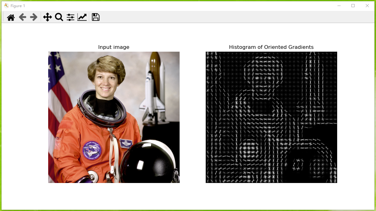
9 # (2) HOG测试:使用Scikit-Image内建的女航天员图像来测试HOG的效果。
10 # 获取测试图片
11 image = data.astronaut()
12
13 # 取得图片的 hog
14 # 参数:ndarray-输入图像 orientations-可选方向箱的数量 pixels_per_cell-可选的单元格大小(以像素为单位)
15 # cells_per_block-可选每个块中的单元格数 visualize-同时返回HOG的图像 multichannel-如果为True,则最后一个图像为u的被视为颜色通道
16 fd, hog_image = hog(image, orientations=8, pixels_per_cell=(16, 16),
17 cells_per_block=(1, 1), visualize=True, multichannel=True)
18
19 # 原图与 hog图比较
20 fig, (ax1, ax2) = plt.subplots(1, 2, figsize=(12, 6), sharex=True, sharey=True)
21
22 ax1.axis('off')
23 # ax1.imshow(image, cmap=plt.cm.gray)
24 ax1.imshow(image)
25 ax1.set_title('Input image')
26
27 # 调整对比,让显示比较清楚
28 # skimage.exposure.exposure 模块中的函数,在对图像进行拉伸或者伸缩强度水平后返回修改后的图像,
29 # 输入图像和输出图像的强度范围分别由 in_range 和 out_range 指定,用来拉伸或缩小输入图像的强度范围。
30 hog_image_rescaled = exposure.rescale_intensity(hog_image, in_range=(0, 10))
31
32 ax2.axis('off')
33 ax2.imshow(hog_image_rescaled, cmap=plt.cm.gray)
34 ax2.set_title('Histogram of Oriented Gradients')
35 # plt.show()
36
37 # (3) 收集正样本:使用scikit-learn内建的人脸数据集作为正样本,共有13233个。
38 # 收集正样本 (positive set)
39 # 使用 scikit-learn 的人脸资料集
40 from sklearn.datasets import fetch_lfw_people
41 faces = fetch_lfw_people()
42 positive_patches = faces.images
43 print("正样本数据大小 = ", positive_patches.shape)
44
45 # (4) 观察正样本中部分图片
46 # 显示正样本部份图片
47 fig, ax = plt.subplots(4, 6)
48 fig.suptitle('image for positive patches', fontsize=14)
49 for i, axi in enumerate(ax.flat):
50 axi.imshow(positive_patches[500 * i], cmap='gray')
51 axi.axis('off')
52
53 # (5)收集负样本 (negative set),使用Scikit-Image内建的数据集,共有9批
54 # 使用 Scikit-Image 的非人脸资料
55 from skimage import data, transform, color
56
57 imgs_to_use = ['hubble_deep_field', 'text', 'coins', 'moon',
58 'page', 'clock', 'coffee', 'chelsea', 'horse']
59 # images = [color.rgb2gray(getattr(data, name)()) for name in imgs_to_use]
60 images = []
61 for na in imgs_to_use:
62 temp = getattr(data, na)()
63 if len(temp.shape) == 3:
64 images.append(color.rgb2gray(temp))
65 else:
66 images.append(color.rgb2gray(color.gray2rgb(temp)))
67
68 print("负样本种类数量 = ", len(images))
69
70 # (6)增加负样本批数:将负样本转换为不同的尺寸,也可以使用数据增补技术。
71 # 将负样本转换为不同的尺寸
72 from sklearn.feature_extraction.image import PatchExtractor
73
74
75 # 转换为不同的尺寸
76 def extract_patches(img, N, scale=1.0, patch_size=positive_patches[0].shape):
77 extracted_patch_size = tuple((scale * np.array(patch_size)).astype(int))
78 # PatchExtractor:产生不同尺寸的图像
79 # PatchExtractor - 从图像集合中提取补丁 patch_size - 一个补丁的尺寸 max_patches - 每幅图像要提取的最补丁数
80 # random_state - 确定 max_patches is not None 时用于随机采样的随机数生成器
81 extractor = PatchExtractor(patch_size=extracted_patch_size, max_patches=N, random_state=0)
82 # Transform the image samples in X into a matrix of patch data.
83 patches = extractor.transform(img[np.newaxis]) # np.newaxis会增加新的一维数据
84 if scale != 1:
85 # skimage.transform.resize图片后会顺便把图片的像素归一化缩放到(0,1)区间内
86 patches = np.array([transform.resize(patch, patch_size) for patch in patches])
87 return patches
88
89
90 # 产生 27000 张图像
91 negative_patches = np.vstack([extract_patches(im, 1000, scale) for im in images for scale in [0.5, 1.0, 2.0]])
92 print(negative_patches.shape)
93
94 # (7)观察负样本中部分图片
95 # 显示部份负样本
96 fig, ax = plt.subplots(4, 6)
97 fig.suptitle('image for negative patches', fontsize=14)
98 # numpy.ndarray.flat 是将数组转换为1-D的迭代器,flat返回的是一个迭代器,可以用for访问数组每一个元素
99 for i, axi in enumerate(ax.flat):
100 axi.imshow(negative_patches[600 * i], cmap='gray')
101 axi.axis('off')
102
103
104 # (8)合并正样本与负样本
105 from skimage import feature # To use skimage.feature.hog()
106 from itertools import chain
107 # chain可以合并它们以形成一个新的单个列表
108 # X_train是数据,y_train实标签(正样本标签为1,负样本标签为0)
109 X_train = np.array([feature.hog(im) for im in chain(positive_patches, negative_patches)])
110 y_train = np.zeros(X_train.shape[0])
111 y_train[:positive_patches.shape[0]] = 1
112
113 # (9)使用 SVM 进行二分类的训练
114 from sklearn.svm import LinearSVC
115 from sklearn.model_selection import GridSearchCV
116
117 # GridSearchCV:用于对估计器的指定参数值进行详尽搜索。cv确定交叉验证切分策略。
118 # LinearSVC:实现线性支持向量机的分类。
119 # dual参数:选择算法以解决双重或原始优化问题。当n_samples> n_features时,首选dual = False。
120 # C为矫正过度拟合强度的倒数(惩罚系数,用来控制损失函数的惩罚系数,类似于LR中的正则化系数),使用 GridSearchCV 寻求最佳参数值
121 grid = GridSearchCV(LinearSVC(dual=False), {'C': [1.0, 2.0, 4.0, 8.0]}, cv=3)
122 grid.fit(X_train, y_train)
123 print("grid.best_score_ = ", grid.best_score_)
124
125 # (10)取得最佳参数值
126 # C 最佳参数值
127 print("grid.best_params_ = ", grid.best_params_)
128
129 # (11)依最佳参数值再训练一次,取得最终模型
130 model = grid.best_estimator_
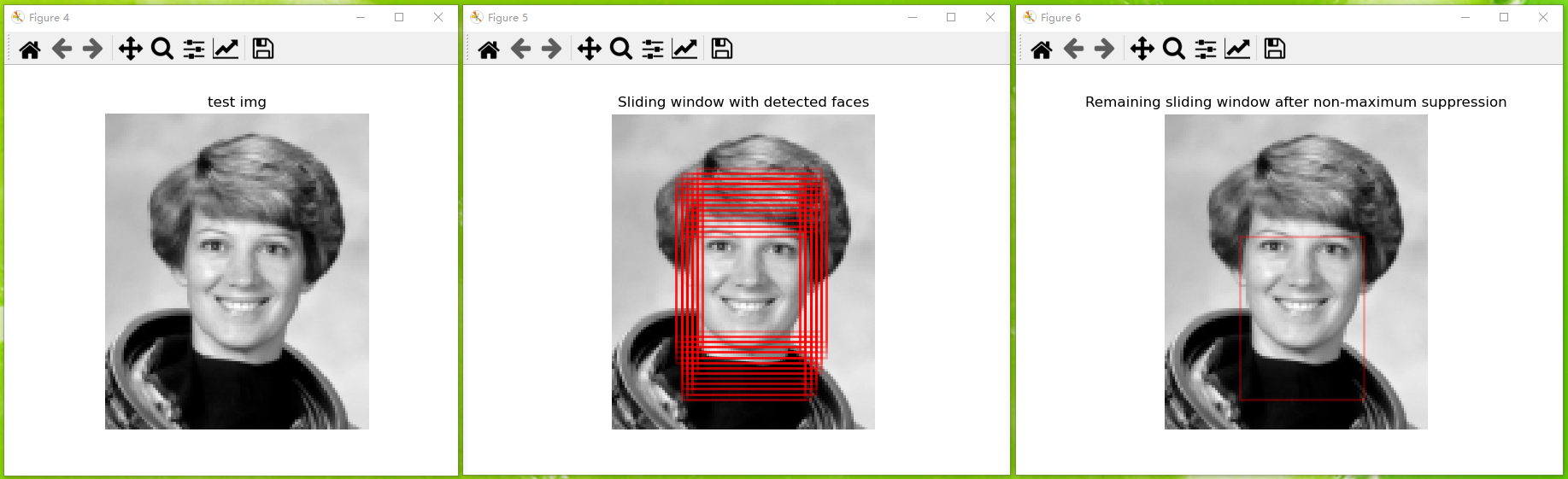
131 model.fit(X_train, y_train)
132
133 # (12)取新图像测试:需先转换为灰阶图像
134 test_img = data.astronaut()
135 test_img = color.rgb2gray(test_img)
136 test_img = transform.rescale(test_img, 0.5) # 对图像进行缩放,参数是缩放的倍数
137 test_img = test_img[:120, 60:160]
138 plt.figure()
139 plt.imshow(test_img, cmap='gray')
140 plt.title('test img')
141 plt.axis('off')
142
143
144 # (13)定义滑动窗口函数
145 # 滑动视窗函数
146 def sliding_window(img, patch_size=positive_patches[0].shape, istep=2, jstep=2, scale=1.0):
147 Ni, Nj = (int(scale * s) for s in patch_size)
148 for i in range(0, img.shape[0] - Ni, istep):
149 for j in range(0, img.shape[1] - Ni, jstep):
150 patch = img[i:i + Ni, j:j + Nj]
151 if scale != 1:
152 patch = transform.resize(patch, patch_size)
153 yield (i, j), patch # (i, j)左上角坐标,patch是裁剪出来互动窗口图片,图片大小是(Ni, Nj)
154
155
156 # (14)计算HOG: 使用滑动窗口来计算每一滑动窗口的 Hog,导入模型辨识
157 indices, patches = zip(*sliding_window(test_img))
158 patches_hog = np.array([feature.hog(patch) for patch in patches])
159 print("patches_hog.shape = ", patches_hog.shape)
160
161 # 辨识每一视窗
162 labels = model.predict(patches_hog)
163 print(labels.sum()) # 侦测到的总数
164
165 # (15)显示这55个合格窗口
166 # 将每一个侦测到的视窗显示出来
167 fig, ax = plt.subplots()
168 ax.imshow(test_img, cmap='gray')
169 ax.set_title('Sliding window with detected faces')
170 ax.axis('off')
171 # 取得左上角座标
172 Ni, Nj = positive_patches[0].shape
173 indices = np.array(indices)
174 # 显示标签为正样本的框
175 for i, j in indices[labels == 1]:
176 # class matplotlib.patches.Rectangle(xy, width, height, *, angle=0.0, rotation_point='xy', **kwargs)
177 ax.add_patch(plt.Rectangle((j, i), Nj, Ni, edgecolor='red', alpha=0.3, lw=2, facecolor='none'))
178 candidate_patches = patches_hog[labels == 1]
179 print("candidate_patches.shape = ", candidate_patches.shape)
180
181
182 # (16)筛选合格窗口:使用Non-Maximum Suppression(NMS) 算法,剔除多余的窗口。
183 # 定义NMS算法函数:这是由Pedro Felipe Felzenszwalb等学者发明的算法,执行速度较慢,Tomasz Malisiewicz因此提出了改善的算法。函数的
184 # 重叠比例阈值(OverlapThresh)参数一般设为0.3~0.5
185 # Non-Maximum Suppression演算法
186 # https://www.pyimagesearch.com/2014/11/17/non-maximum-suppression-object-detection-python/
187 # Non-Maximum Suppression演算法 by Felzenszwalb et al.
188 # boxes:所有候选的视窗,overlapThresh:视窗重叠的比例门槛
189 def non_max_suppression_slow(boxes, overlapThresh=0.5):
190 if len(boxes) == 0:
191 return []
192
193 pick = [] # 储存筛选的结果
194 x1 = boxes[:, 0] # 取得候选的视窗的左/上/右/下 坐标
195 y1 = boxes[:, 1]
196 x2 = boxes[:, 2]
197 y2 = boxes[:, 3]
198
199 # 计算候选视窗的面积
200 area = (x2 - x1 + 1) * (y2 - y1 + 1)
201 idxs = np.argsort(y2) # 依视窗的底Y座标排序
202
203 # 比对重叠比例
204 while len(idxs) > 0:
205 # 最后一笔
206 last = len(idxs) - 1
207 i = idxs[last]
208 pick.append(i)
209 suppress = [last]
210
211 # 比对最后一笔与其他视窗重叠的比例
212 for pos in range(0, last):
213 j = idxs[pos]
214 print(i, j)
215 print("i = ", x1[i], y1[i], x2[i], y2[i], "j = ", x1[j], y1[j], x2[j], y2[j])
216 # 取得所有视窗的涵盖范围
217 xx1 = max(x1[i], x1[j])
218 yy1 = max(y1[i], y1[j])
219 xx2 = min(x2[i], x2[j])
220 yy2 = min(y2[i], y2[j])
221 w = max(0, xx2 - xx1 + 1)
222 h = max(0, yy2 - yy1 + 1)
223 # _, (ax1, ax2) = plt.subplots(1, 2)
224 # ax1.imshow(test_img, cmap='gray')
225 # ax1.axis('off')
226 # ax1.add_patch(plt.Rectangle((x1[i], y1[i]), Nj, Ni, edgecolor='red', alpha=0.3, lw=2, facecolor='none'))
227 # ax1.add_patch(plt.Rectangle((x1[j], y1[j]), Nj, Ni, edgecolor='blue', alpha=0.3, lw=2, facecolor='none'))
228 # ax2.imshow(test_img, cmap='gray')
229 # ax2.axis('off')
230 # ax2.add_patch(plt.Rectangle((xx1, yy1), xx2-xx1, yy2-yy1, edgecolor='Magenta', alpha=0.3, lw=2, facecolor='none'))
231
232 # 计算重叠比例
233 overlap = float(w * h) / area[j]
234 print("overlap = ", overlap)
235 # 如果大于门槛值,则储存起来
236 if overlap > overlapThresh:
237 suppress.append(pos)
238 # print("suppress = ", suppress)
239 pass
240 # 删除合格的视窗,继续比对
241 idxs = np.delete(idxs, suppress) # 在这里删除之后,idxs就为array([], dtype=int64)
242
243 # 传回合格的视窗
244 return boxes[pick]
245
246
247 # (17)呼叫 non_max_suppression_slow 函数,剔除处于的窗口
248 # 使用 Non-Maximum Suppression演算法,剔除多余的视窗。
249 candidate_boxes = []
250 for i, j in indices[labels == 1]:
251 candidate_boxes.append([j, i, Nj+j, Ni+i])
252 final_boxes = non_max_suppression_slow(np.array(candidate_boxes).reshape(-1, 4))
253
254 # 将每一个合格的视窗显示出来
255 fig, ax = plt.subplots()
256 ax.imshow(test_img, cmap='gray')
257 ax.set_title('Remaining sliding window after non-maximum suppression')
258 ax.axis('off')
259 # 显示
260 for x1, y1, x2, y2 in final_boxes:
261 ax.add_patch(plt.Rectangle((x1, y1), x2-x1, y2-y1, edgecolor='red', alpha=0.3, lw=2, facecolor='none'))
262 pass
注意:
1. matplotlib 在交互模式下想要显示图片内容且可以看变量的参数,可以在 262 行打上断点,就可以看到图片了。
2. 在非极大值抑制算法中,我们本应该要根据每个 boundingbox 的置信度得分排列 boundingbox,拿置信度得分最高的 boundingbox 和其他的 boundingbox 进行比较从而剔除和最高置信度得分的 boundingbox 重叠程度超过一定阈值的 boundingbox,但是这里使用的是选择右下角坐标 y 值最大的值作为第一个保留项,这里和实际的 NMS是不一样的。
运行结果:


 浙公网安备 33010602011771号