

# libraries we'll need
library(car) # for avplots
library(tidyverse) # for general utility functions

# read in our data
bmi_data <- read_csv("../input/eating-health-module-dataset//ehresp_2014.csv") %>%
    filter(erbmi > 0) # remove rows where the reported BMI is less than 0 (impossible)
nyc_census <- read_csv("../input/new-york-city-census-data/nyc_census_tracts.csv")
# fit a glm model
model <- glm(erbmi ~ euexfreq + euwgt + euhgt + ertpreat, # formula
             data = bmi_data, # dataset
             family = ("gaussian")) # fit a linear model
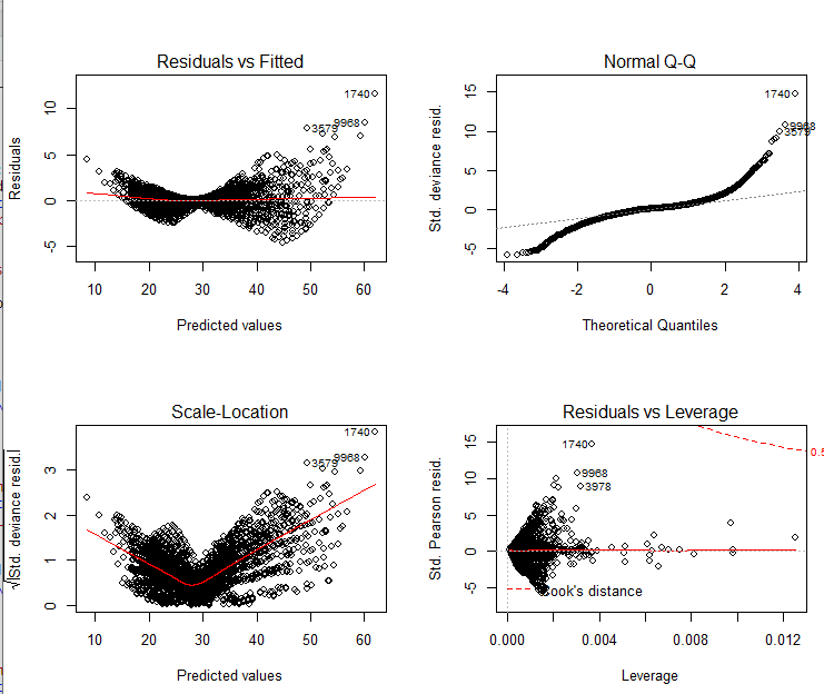
# output plots in a 2 x 2 grid
par(mfrow = c(2,2))
# diagnostic plots
plot(model)
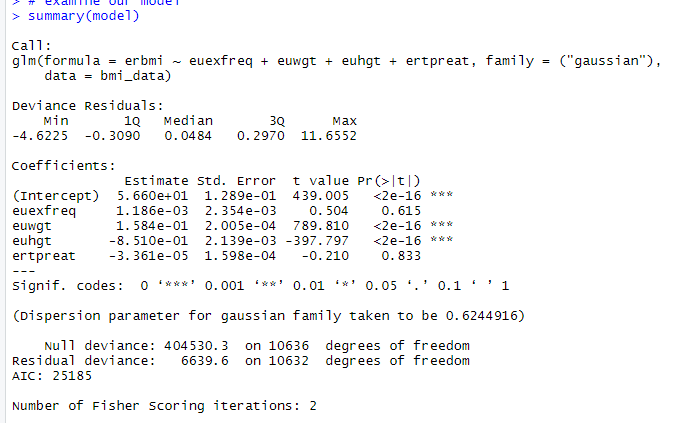
# examine our model
summary(model)
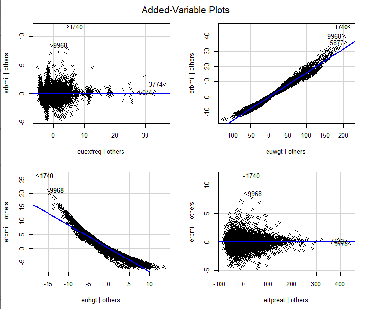
# added-variable plots for our model
avPlots(model)
结论
看这些图,我们可以在右上角看到随着euwgt(体重)的增加,erbmi(体重指数,我们试图预测的变量)也在增加。看左下角我们可以看到,随着euhgt(高度)的增加,erbmi实际上在减少。所以身高和体重都很重要,但它们有相反的效果!我们也可以从模型总结中看出这一点,因为euwgt的估计值为正,而euhgt的估计值为负。
另外两个图显示这些变量和我们要预测的变量之间没有很强的关系,我们已经从模型中算出来了。
