


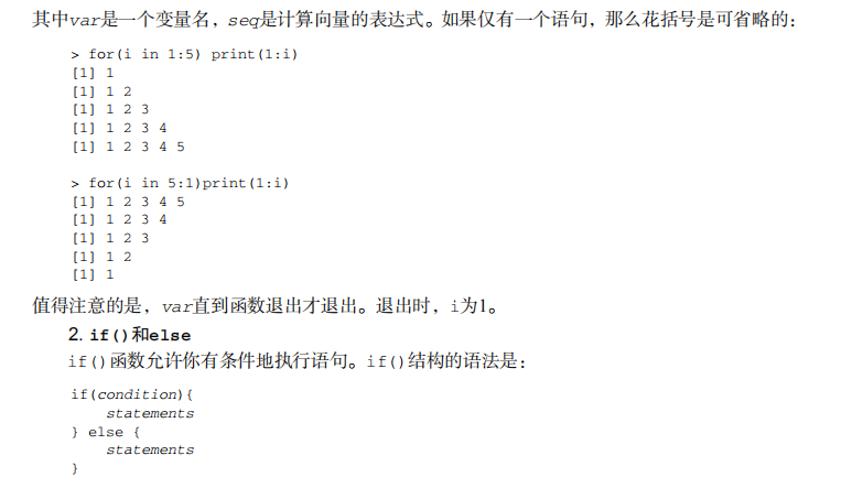
运行的条件是一元逻辑向量(TRUE或FALSE)并且不能有缺失(NA)。else部分是可选的。如果 13
仅有一个语句,花括号也是可以省略的。
下面的代码片段是一个例子:
if(interactive()){ 14
 plot(x, y)
} else {
 png("myplot.png")
 plot(x, y)
 dev.off() 15
}
如果代码交互运行,interactive()函数返回TRUE,同时输出一个曲线图。否则,曲线图被存
在磁盘里。你可以使用第21章中的if()函数。 16
3. ifelse()
ifelse()是函数if()的量化版本。矢量化允许一个函数来处理没有明确循环的对象。
ifelse()的格式是: 17
ifelse(test, yes, no)
其中test是已强制为逻辑模式的对象,yes返回test元素为真时的值,no返回test元素为假时
的值。 18
比如你有一个p值向量,是从包含六个统计检验的统计分析中提取出来的,并且你想要标记
p<0.05水平下的显著性检验。可以使用下面的代码:
> pvalues <- c(.0867, .0018, .0054, .1572, .0183, .5386) 19
> results <- ifelse(pvalues <.05, "Significant", "Not Significant")
> results
[1] "Not Significant" "Significant" "Significant"
[4] "Not Significant" "Significant" "Not Significant" 20
ifelse()函数通过pvalues向量循环并返回一个包括"Significant"或"Not Significant"
的字符串。返回的结果依赖于pvalues返回的值是否大于0.05。
同样的结果可以使用显式循环完成: 21
pvalues <- c(.0867, .0018, .0054, .1572, .0183, .5386)
results <- vector(mode="character", length=length(pvalues))
for(i in 1:length(pvalues)){ 22
 if (pvalues[i] < .05) results[i] <- "Significant"
 else results[i] <- "Not Significant"
}
可以看出,向量化的版本更快且更有效。 23
有一些其他的控制结构,包括while()、repeat()和switch(),但是这里介绍的是最常用
的。有了数据结构和控制结构,我们就可以讨论创建函数了。
20.1.3 创建函数
在R中处处是函数。算数运算符+、-、/和*实际上也是函数。例如,2 + 2等价于 "+"(2, 2)。
本节将主要描述函数语法。语句环境将在20-2节描述。
1. 函数语法
函数的语法格式是:
functionname <- function(parameters){
statements
 return(value)
}
如果函数中有多个参数,那么参数之间用逗号隔开。
参数可以通过关键字和/或位置来传递。另外,参数可以有默认值。请看下面的函数:
f <- function(x, y, z=1){
 result <- x + (2*y) + (3*z)
 return(result)
}
> f(2,3,4)
[1] 20
> f(2,3)
[1] 11
> f(x=2, y=3)
[1] 11
> f(z=4, y=2, 3)
[1] 19
在第一个例子中,参数是通过位置(x=2,y=3,z=4)传递的。在第二个例子中,参数也是通过
位置传递的,并且z默认为1。在第三个例子中,参数是通过关键字传递的,z也默认为1。在最后
一个例子中,y和z是通过关键字传递的,并且x被假定为未明确指定的(这里x=3)第一个参数。
参数是可选的,但即使没有值被传递也必须使用圆括号。return()函数返回函数产生的对
象。它也是可选的;如果缺失,函数中最后一条语句的结果也会被返回。
你可以使用args()函数来观测参数的名字和默认值:
> args(f)
 function (x, y, z = 0)
 NULL
args()被设计用于交互式观测。如果你需要以编程方式获取参数名称和默认值,可以使用
formals()函数。它返回含有必要信息的列表。
参数是按值传递的,而不是按地址传递。请看下面这个函数语句:
result <- lm(height ~ weight, data=women)
women数据集不是直接得到的。需要形成一个副本然后传递给函数。如果women数据集很大的话,
内存(RAM)可能被迅速用完。这可能成为处理大数据问题时的难题能需要使用特殊的技术(见


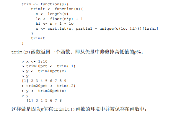

#--------------------------------------------------------------------#
# R in Action (2nd ed): Chapter 20                                   #
# Advanced R programming                                             #
# requires packages ggplot2, reshape2, foreach, doParallel           #
# install.packages(c("ggplot2", "reshap2e", "foreach", "doParallel"))#
#--------------------------------------------------------------------#

# Atomic vectors
passed <- c(TRUE, TRUE, FALSE, TRUE)
ages <- c(15, 18, 25, 14, 19)
cmplxNums <- c(1+2i, 0+1i, 39+3i, 12+2i)
names <- c("Bob", "Ted", "Carol", "Alice")


# Matrices
x <- c(1,2,3,4,5,6,7,8)
class(x)
print(x)
attr(x, "dim") <- c(2,4)
print(x)
class(x)
attributes(x)
attr(x, "dimnames") <- list(c("A1", "A2"),
                            c("B1", "B2", "B3", "B4"))
print(x)
attr(x, "dim") <- NULL
class(x)
print(x)


# Generic vectors (lists)
head(iris)
unclass(iris)
attributes(iris)

set.seed(1234)
fit <- kmeans(iris[1:4], 3)
names(fit)
unclass(fit)
sapply(fit, class)

# Indexing atomic vectors
x <- c(20, 30, 40)
x[3]
x[c(2,3)]
x <- c(A=20, B=30, C=40)
x[c(2,3)]
x[c("B", "C")]


# Indexing lists
fit[c(2,7)]
fit[2]
fit[[2]]
fit$centers
fit[[2]][1,]
fit$centers$Petal.Width  # should give an error


# Listing 20.1 - Plotting the centroides from a k-mean cluster analysis
fit <- kmeans(iris[1:4], 3)
means <- fit$centers
library(reshape2)
dfm <- melt(means)
names(dfm) <- c("Cluster", "Measurement", "Centimeters")
dfm$Cluster <- factor(dfm$Cluster)
head(dfm)
library(ggplot2)
ggplot(data=dfm,
       aes(x=Measurement, y=Centimeters, group=Cluster)) +
  geom_point(size=3, aes(shape=Cluster, color=Cluster)) +
  geom_line(size=1, aes(color=Cluster)) +
  ggtitle("Profiles for Iris Clusters")


# for loops
for(i in 1:5) print(1:i)
for(i in 5:1)print(1:i)

# ifelse
pvalues <- c(.0867, .0018, .0054, .1572, .0183, .5386)
results <- ifelse(pvalues <.05, "Significant", "Not Significant")
results

pvalues <- c(.0867, .0018, .0054, .1572, .0183, .5386)
results <- vector(mode="character", length=length(pvalues))
for(i in 1:length(pvalues)){
  if (pvalues[i] < .05) results[i] <- "Significant"
  else results[i] <- "Not Significant"
}
results

# Creating functions
f <- function(x, y, z=1){
  result <- x + (2*y) + (3*z)
  return(result)
}

f(2,3,4)
f(2,3)
f(x=2, y=3)
f(z=4, y=2, 3)
args(f)


# object scope
x <- 2
y <- 3
z <- 4
f <- function(w){
  z <- 2
  x <- w*y*z
  return(x)
}
f(x)
x
y
z


# Working with environments
x <- 5
myenv <- new.env()
assign("x", "Homer", env=myenv)
ls()
ls(myenv)
x
get("x", env=myenv)

myenv <- new.env()
myenv$x <- "Homer"
myenv$x

parent.env(myenv)


# function closures
trim <- function(p){
  trimit <- function(x){
    n <- length(x)
    lo <- floor(n*p) + 1
    hi <- n + 1 - lo
    x <- sort.int(x, partial = unique(c(lo, hi)))[lo:hi]
  }
  trimit
}
x <- 1:10
trim10pct <- trim(.1)
y <- trim10pct(x)
y
trim20pct <- trim(.2)
y <- trim20pct(x)
y

ls(environment(trim10pct))
get("p", env=environment(trim10pct))

makeFunction <- function(k){
  f <- function(x){
    print(x + k)
  }
}

g <- makeFunction(10)
g (4)
k <- 2
g (5)

ls(environment(g))
environment(g)$k


# Generic functions
summary(women)
fit <- lm(weight ~ height, data=women)
summary(fit)

class(women)
class(fit)
methods(summary)


# Listing 20.2 - An example of a generic function
mymethod <- function(x, ...) UseMethod("mymethod")
mymethod.a <- function(x) print("Using A")
mymethod.b <- function(x) print("Using B")
mymethod.default <- function(x) print("Using Default")

x <- 1:5
y <- 6:10
z <- 10:15
class(x) <- "a"
class(y) <- "b"

mymethod(x)
mymethod(y)
mymethod(z)

class(z) <- c("a", "b")
mymethod(z)
class(z) <- c("c", "a", "b")
mymethod(z)


# Vectorization and efficient code
set.seed(1234)
mymatrix <- matrix(rnorm(10000000), ncol=10)
accum <- function(x){
  sums <- numeric(ncol(x))
  for (i in 1:ncol(x)){
    for(j in 1:nrow(x)){
      sums[i] <- sums[i] + x[j,i]
    }
  }
}
system.time(accum(mymatrix))   # using loops
system.time(colSums(mymatrix)) # using vectorization


# Correctly size objects
set.seed(1234)
k <- 100000
x <- rnorm(k)

y <- 0
system.time(for (i in 1:length(x)) y[i] <- x[i]^2)

y <- numeric(k)
system.time(for (i in 1:k) y[i] <- x[i]^2)

y <- numeric(k)
system.time(y <- x^2)

# Listing 20.3 - Parallelization with foreach and doParallel
library(foreach)
library(doParallel)
registerDoParallel(cores=4)

eig <- function(n, p){
  x <- matrix(rnorm(100000), ncol=100)
  r <- cor(x)
  eigen(r)$values
}
n <- 1000000
p <- 100
k <- 500


system.time(
  x <- foreach(i=1:k, .combine=rbind) %do% eig(n, p)
)

system.time(
  x <- foreach(i=1:k, .combine=rbind) %dopar% eig(n, p)
)

# Finding common errors
mtcars$Transmission <- factor(mtcars$a,
                              levels=c(1,2),
                              labels=c("Automatic", "Manual"))
aov(mpg ~ Transmission, data=mtcars) # generates error
head(mtcars[c("mpg", "Transmission")])
table(mtcars$Transmission) # here is the source of the error

# Listing 20.4 - A sample debugging session
args(mad)
debug(mad)
mad(1:10)
# enters debugging mode
# Q to quit - see text
undebug(mad)


# Listing 20.5 - Sample debugging session with recover()
f <- function(x, y){
  z <- x + y
  g(z)
}
g <- function(x){
  z <- round(x)
  h(z)
}

h <- function(x){
  set.seed(1234)
  z <- rnorm(x)
  print(z)
}
options(error=recover)

f(2,3)
f(2, -3) # enters debugging mode at this point
