# 导入模块,并重命名为np
import numpy as np
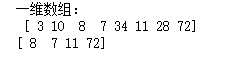
# 单个列表创建一维数组
arr1 = np.array([3,10,8,7,34,11,28,72])
print('一维数组:\n',arr1)
# 一维数组元素的获取
print(arr1[[2,3,5,7]])
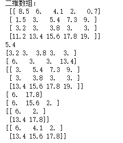
# 嵌套元组创建二维数组
arr2 = np.array(((8.5,6,4.1,2,0.7),(1.5,3,5.4,7.3,9),(3.2,3,3.8,3,3),(11.2,13.4,15.6,17.8,19)))
print('二维数组:\n',arr2)
# 二维数组元素的获取
# 第2行第3列元素
print(arr2[1,2])
# 第3行所有元素
print(arr2[2,:])
# 第2列所有元素
print(arr2[:,1])
# 第2至4行,2至5行
print(arr2[1:4,1:5])
# 第一行、最后一行和第二列、第四列构成的数组
print(arr2[[0,-1],[1,3]])
# 第一行、最后一行和第一列、第三列、第四列构成的数组
print(arr2[[0,-1,0],[1,2,3]])
# 第一行、最后一行和第二列、第四列构成的数组
print(arr2[np.ix_([0,-1],[1,3])])
# 第一行、最后一行和第一列、第三列、第四列构成的数组
print(arr2[np.ix_([0,-1],[1,2,3])])
# 读入数据
stu_score = np.genfromtxt(fname = r'F:\\python_Data_analysis_and_mining\\04\\stu_socre.txt',delimiter='\t',skip_header=1)
# 查看数据结构
print(type(stu_score))
# 查看数据维数
print(stu_score.ndim)
# 查看数据行列数
print(stu_score.shape)
# 查看数组元素的数据类型
print(stu_score.dtype)
# 查看数组元素个数
print(stu_score.size)

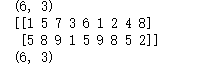
arr3 = np.array([[1,5,7],[3,6,1],[2,4,8],[5,8,9],[1,5,9],[8,5,2]])
# 数组的行列数
print(arr3.shape)
# 使用reshape方法更改数组的形状
print(arr3.reshape(2,9))
# 打印数组arr3的行列数
print(arr3.shape)
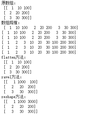
arr4 = np.array([[1,10,100],[2,20,200],[3,30,300]])
print('原数组:\n',arr4)
# 默认排序降维
print('数组降维:\n',arr4.ravel())
print(arr4.flatten())
print(arr4.reshape(-1))
# 改变排序模式的降维
print(arr4.ravel(order = 'F'))
print(arr4.flatten(order = 'F'))
print(arr4.reshape(-1, order = 'F'))
# 更改预览值
arr4.flatten()[0] = 2000
print('flatten方法:\n',arr4)
arr4.ravel()[1] = 1000
print('ravel方法:\n',arr4)
arr4.reshape(-1)[2] = 3000
print('reshape方法:\n',arr4)
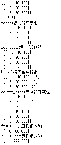
arr4 = np.array([[1,10,100],[2,20,200],[3,30,300]])
arr5 = np.array([1,2,3])
print(arr4)
print(arr5)
print('vstack纵向合并数组:\n',np.vstack([arr4,arr5]))
print('row_stack纵向合并数组:\n',np.row_stack([arr4,arr5]))
arr6 = np.array([[5],[15],[25]])
print('hstack横向合并数组:\n',np.hstack([arr4,arr6]))
print('column_stack横向合并数组:\n',np.column_stack([arr4,arr6]))
print(arr4)
print('垂直方向计算数组的和:\n',np.sum(arr4,axis = 0))
print('水平方向计算数组的和:\n',np.sum(arr4, axis = 1))
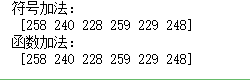
# 加法运算
math = np.array([98,83,86,92,67,82])
english = np.array([68,74,66,82,75,89])
chinese = np.array([92,83,76,85,87,77])
tot_symbol = math+english+chinese
tot_fun = np.add(np.add(math,english),chinese)
print('符号加法:\n',tot_symbol)
print('函数加法:\n',tot_fun)
# 除法运算
height = np.array([165,177,158,169,173])
weight = np.array([62,73,59,72,80])
BMI_symbol = weight/(height/100)**2
BMI_fun = np.divide(weight,np.divide(height,100)**2)
print('符号除法:\n',BMI_symbol)
print('函数除法:\n',BMI_fun)

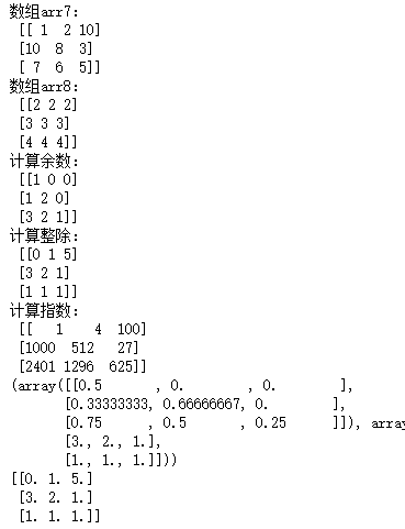
arr7 = np.array([[1,2,10],[10,8,3],[7,6,5]])
arr8 = np.array([[2,2,2],[3,3,3],[4,4,4]])
print('数组arr7:\n',arr7)
print('数组arr8:\n',arr8)
# 求余数
print('计算余数:\n',arr7 % arr8)
# 求整除
print('计算整除:\n',arr7 // arr8)
# 求指数
print('计算指数:\n',arr7 ** arr8)
print(np.modf(arr7/arr8))
# 整除部分
print(np.modf(arr7/arr8)[1])
arr7 = np.array([[1,2,10],[10,8,3],[7,6,5]])
arr8 = np.array([[2,2,2],[3,3,3],[4,4,4]])
print('数组arr7:\n',arr7)
print('数组arr8:\n',arr8)
# 取子集
# 从arr7中取出arr7大于arr8的所有元素
print('满足条件的二维数组元素获取:\n',arr7[arr7>arr8])
# 从arr9中取出大于10的元素
arr9 = np.array([3,10,23,7,16,9,17,22,4,8,15])
print('满足条件的一维数组元素获取:\n',arr9[arr9>10])

# 判断操作
# 将arr7中大于7的元素改成5,其余的不变
print('二维数组的条件操作:\n',np.where(arr7>7,5,arr7))
# 将arr9中大于10 的元素改为1,否则改为0
print('一维数组的条件操作:\n',np.where(arr9>10,1,0))

# 各输入数组维度一致,对应维度值相等
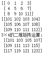
arr10 = np.arange(12).reshape(3,4)
print(arr10)
arr11 = np.arange(101,113).reshape(3,4)
print(arr11)
print('3×4的二维矩阵运算:\n',arr10 + arr11)
# 各输入数组维度不一致,对应维度值相等
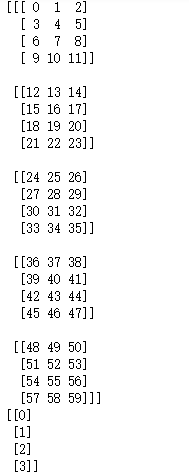
arr12 = np.arange(60).reshape(5,4,3)
print(arr12)
arr10 = np.arange(12).reshape(4,3)
print(arr10)
print('维数不一致,但末尾的维度值一致:\n',arr12 + arr10)

# 各输入数组维度不一致,对应维度值不相等,但其中有一个为1
arr12 = np.arange(60).reshape(5,4,3)
print(arr12)
arr13 = np.arange(4).reshape(4,1)
print(arr13)
print('维数不一致,维度值也不一致,但维度值至少一个为1:\n',arr12 + arr13)
# 加1补齐
arr14 = np.array([5,15,25])
print('arr14的维度自动补齐为(1,3):\n',arr10 + arr14)
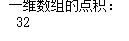
# 一维数组的点积
vector_dot = np.dot(np.array([1,2,3]), np.array([4,5,6]))
print('一维数组的点积:\n',vector_dot)
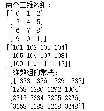
# 二维数组的乘法
print('两个二维数组:')
print(arr10)
print(arr11)
arr2d = np.dot(arr10,arr11)
print('二维数组的乘法:\n',arr2d)
import numpy as np
# diag的使用
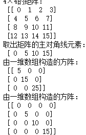
arr15 = np.arange(16).reshape(4,-1)
print('4×4的矩阵:\n',arr15)
print('取出矩阵的主对角线元素:\n',np.diag(arr15))
print('由一维数组构造的方阵:\n',np.diag(np.array([5,15,25])))
print('由一维数组构造的方阵:\n',np.diag(np.array(np.diag(arr15))))
# 计算方阵的特征向量和特征根
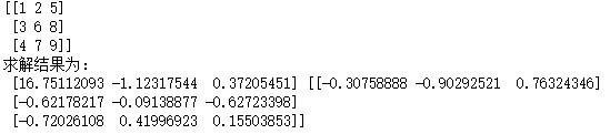
arr16 = np.array([[1,2,5],[3,6,8],[4,7,9]])
print(arr16)
a,b = np.linalg.eig(arr16)
print('求解结果为:\n',a,b)
# 计算偏回归系数
X = np.array([[1,1,4,3],[1,2,7,6],[1,2,6,6],[1,3,8,7],[1,2,5,8],[1,3,7,5],[1,6,10,12],[1,5,7,7],[1,6,3,4],[1,5,7,8]])
print(X)
print(X.shape)
Y = np.array([3.2,3.8,3.7,4.3,4.4,5.2,6.7,4.8,4.2,5.1])
print(Y)
print(Y.shape)
X_trans_X_inverse = np.linalg.inv(np.dot(np.transpose(X),X))
print(X_trans_X_inverse)
beta = np.dot(np.dot(X_trans_X_inverse,np.transpose(X)),Y)
print('偏回归系数为:\n',beta)

# 多元线性方程组
A = np.array([[3,2,1],[2,3,1],[1,2,3]])
print(A)
b = np.array([39,34,26])
print(b)
X = np.linalg.solve(A,b)
print('三元一次方程组的解:\n',X)

# 范数的计算
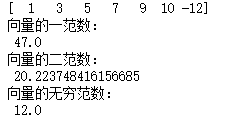
arr17 = np.array([1,3,5,7,9,10,-12])
print(arr17)
# 一范数
res1 = np.linalg.norm(arr17, ord = 1)
print('向量的一范数:\n',res1)
# 二范数
res2 = np.linalg.norm(arr17, ord = 2)
print('向量的二范数:\n',res2)
# 无穷范数
res3 = np.linalg.norm(arr17, ord = np.inf)
print('向量的无穷范数:\n',res3)
import seaborn as sns
import matplotlib.pyplot as plt
from scipy import stats
# 生成各种正态分布随机数
np.random.seed(1234)
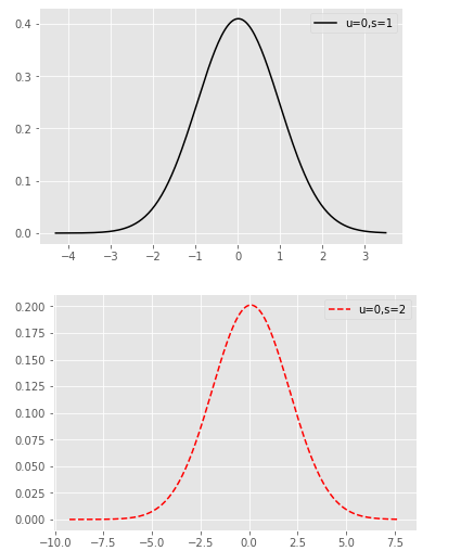
rn1 = np.random.normal(loc = 0, scale = 1, size = 1000)
print(rn1.shape)
rn2 = np.random.normal(loc = 0, scale = 2, size = 1000)
print(rn2.shape)
rn3 = np.random.normal(loc = 2, scale = 3, size = 1000)
print(rn3.shape)
rn4 = np.random.normal(loc = 5, scale = 3, size = 1000)
print(rn4.shape)
# 绘图
plt.style.use('ggplot')
sns.distplot(rn1, hist = False, kde = False, fit = stats.norm, fit_kws = {'color':'black','label':'u=0,s=1','linestyle':'-'})
# 呈现图例
plt.legend()
plt.show()
sns.distplot(rn2, hist = False, kde = False, fit = stats.norm, fit_kws = {'color':'red','label':'u=0,s=2','linestyle':'--'})
# 呈现图例
plt.legend()
plt.show()
sns.distplot(rn3, hist = False, kde = False, fit = stats.norm, fit_kws = {'color':'blue','label':'u=2,s=3','linestyle':':'})
# 呈现图例
plt.legend()
plt.show()
sns.distplot(rn4, hist = False, kde = False, fit = stats.norm, fit_kws = {'color':'purple','label':'u=5,s=3','linestyle':'-.'})
# 呈现图例
plt.legend()
plt.show()
import seaborn as sns
import matplotlib.pyplot as plt
from scipy import stats
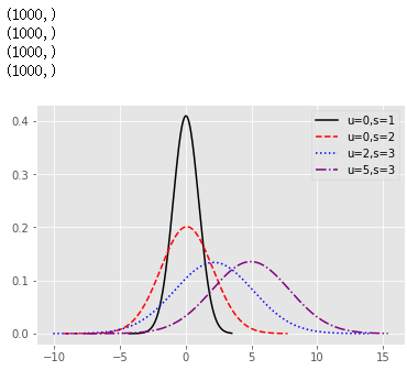
# 生成各种正态分布随机数
np.random.seed(1234)
rn1 = np.random.normal(loc = 0, scale = 1, size = 1000)
print(rn1.shape)
rn2 = np.random.normal(loc = 0, scale = 2, size = 1000)
print(rn2.shape)
rn3 = np.random.normal(loc = 2, scale = 3, size = 1000)
print(rn3.shape)
rn4 = np.random.normal(loc = 5, scale = 3, size = 1000)
print(rn4.shape)
# 绘图
plt.style.use('ggplot')
sns.distplot(rn1, hist = False, kde = False, fit = stats.norm, fit_kws = {'color':'black','label':'u=0,s=1','linestyle':'-'})
sns.distplot(rn2, hist = False, kde = False, fit = stats.norm, fit_kws = {'color':'red','label':'u=0,s=2','linestyle':'--'})
sns.distplot(rn3, hist = False, kde = False, fit = stats.norm, fit_kws = {'color':'blue','label':'u=2,s=3','linestyle':':'})
sns.distplot(rn4, hist = False, kde = False, fit = stats.norm, fit_kws = {'color':'purple','label':'u=5,s=3','linestyle':'-.'})
# 呈现图例
plt.legend()
plt.show()
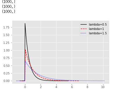
# 生成各种指数分布随机数
np.random.seed(1234)
re1 = np.random.exponential(scale = 0.5, size = 1000)
re2 = np.random.exponential(scale = 1, size = 1000)
re3 = np.random.exponential(scale = 1.5, size = 1000)
print(re1.shape)
print(re2.shape)
print(re3.shape)
# 绘图
sns.distplot(re1, hist = False, kde = False, fit = stats.expon,
fit_kws = {'color':'black','label':'lambda=0.5','linestyle':'-'})
sns.distplot(re2, hist = False, kde = False, fit = stats.expon,
fit_kws = {'color':'red','label':'lambda=1','linestyle':'--'})
sns.distplot(re3, hist = False, kde = False, fit = stats.expon,
fit_kws = {'color':'blue','label':'lambda=1.5','linestyle':':'})
# 呈现图例
plt.legend()
# 呈现图形
plt.show()