『笔记』OReilly Learning OpenCV

『笔记』OReilly Learning OpenCV

Chapter 6: Image Transforms#

Stretch, Shrink, Warp, and Rotate#

In this section we turn to geometric manipulations of images. Such manipulations include stretching in various ways, which includes both uniform and nonuniform resizing (the latter is known as warping)
We will cover these transformations in detail here; we will return to them when we discuss (in Chapter 11) how they can be used in the context of three-dimensional vision techniques.

The functions that can stretch, shrink, warp, and/or rotate an image are called geometric transforms. For planar areas, there are two flavors of geometric transforms: transforms that use a 2-by-3 matrix, which are called affine transforms; and transforms based on a 3-by-3 matrix, which are called perspective transforms or homographies .

You can think of the latter transformation as a method for computing the way in which a plane in three dimensions is perceived by a particular observer, who might not be looking straight on at that plane.

Note: 在这里，context是对于image的transform处理，也就是对2d平面的处理。其中affine transform就是二维上的[R t]，相当于平行四边形到另一个平行四边形。而perspective transform/homography包含了affine transform，更general也可以实现例如平行四边形到梯形这种不平行的转换，这是因为虽然在这里介绍出了perspective transform/homography，但其实它更属于chapter 11那边三维的范畴，其就是你从一个别的视角去看这个平面所得到新平面，在这里正好可以理解为形成了新image的方式。而推导也是由三维的extrinsic transformation + projection（相机那一套）下由于设置world坐标Z=0下的一个特殊情况实现的仿佛2维到2维的变换（在chapter 11已经完全了解了），换言之，它就是一个三维context下最经典操作extrinsic transformation + projection将三维点转换为像素点的Z=0的特殊情况，而这个特殊情况带来的意义恰好可以符合那里的camera calibration (with chessboard)以及作为这里的image manipulation. 所以在这里来说其实有点降维打击了还在讨论二维上如何变的context，因而能够实现任意的变换

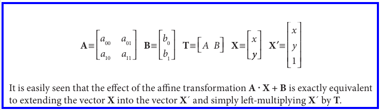
An affine transformation is any transformation that can be expressed in the form of a matrix multiplication followed by a vector addition. In OpenCV the standard style of representing such a transformation is as a 2-by-3 matrix.

• Note: 关于affine这个东西，看到这句话又熟悉起来了，就是乘一个再加一个

• 

• Affine transformations can be visualized as follows. Any parallelogram ABCD in a plane can be mapped to any other parallelogram A'B'C'D' by some affine transformation.

• Affine transforms can convert rectangles to parallelograms. They can squash the shape but must keep the sides parallel; they can rotate it and/or scale it. Perspective transformations offer more flexibility; a perspective transform can turn a rectangle into a trapezoid. Affine transformations are a subset of perspective transformations.

• 

Affine Transform#

Dense affine transformations#

In the first case, the obvious input and output formats are images, and the implicit requirement is that the warping assumes the pixels are a dense representation of the underlying image. This means that image warping must necessarily handle interpolations so that the output images are smooth and look natural.

• Note: 这里是有了map_matrix(2x3 affine transformation)去做变换

• Note: 可以想象，你warp了之后像素点肯定不是正正好好地在grid上，为了形成新的image肯定需要interpolation

cVWarpAffine performance#

cvWarpAffine()

Computing the affine map matrix#

OpenCV provides two functions to help you generate the map_matrix. The first is used when you already have two images that you know to be related by an affine transformation or that you’d like to approximate in that way

The second way to compute the map_matrix is to use cv2DRotationMatrix(), which computes the map matrix for a rotation around some arbitrary point, combined with an optional rescaling. This is just one possible kind of affine transformation.

Sparse affine transformations#

For sparse mappings (i.e., mappings of lists of individual points), it is best to use cvTransform()

Perspective Transform#

First we remark that, even though a perspective projection is specified completely by a single matrix, the projection is not actually a linear transformation. This is because the transformation requires division by the final dimension （确实，真贴心，这更像是一种特殊的操作，只是简练成了matrix的形式）

Dense perspective transform#

Computing the perspective map matrix#

Sparse perspective transformations#

Chapter 11: Camera models and calibration#

Note: 至此关于camera model/projection transform相关的内容已经多处学习过了（slam14/ro47004/CVbyDL/learning opencv），目前可以说自己了解这块知识了。

Vision begins with the detection of light from the world. That light begins as rays emanating from some source (e.g., a light bulb or the sun), which then travels through space until striking some object. When that light strikes the object, much of the light is absorbed, and what is not absorbed we perceive as the color of the light. Reflected light that makes its way to our eye (or our camera) is collected on our retina (or our imager). The geometry of this arrangement—particularly of the ray’s travel from the object, through the lens in our eye or camera, and to the retina or imager—is of particular importance to practical vision.

The process of camera calibration gives us both a model of the camera’s geometry and a distortion model of the lens. These two informational models define the intrinsic parameters of the camera

Camera Model (and lens distortions)#

A simple but useful model of how this happens is the pinhole camera model. A pinhole is an imaginary wall with a tiny hole in the center that blocks all rays except those passing through the tiny aperture in the center

In a physical pinhole camera, this point is then “projected” onto an imaging surface. As a result, the image on this image plane (also called the projective plane ) is always in focus, and the size of the image relative to the distant object is given by a single parameter of the camera: its focal length. For our idealized pinhole camera, the distance from the pinhole aperture to the screen is precisely the focal length.

$$-x=f\frac{X}{Z}$$

Step: swap the pinhole and the image plane. The point in the pinhole is reinterpreted as the center of projection. In this way of looking at things, every ray leaves a point on the distant object and heads for the center of projection.

• The point at the intersection of the image plane and the optical axis is referred to as the principal point.（也就是一个实际中物理上的定义）

• The image plane is really just the projection screen “pushed” in front of the pinhole. The image plane is simply a way of thinking of a “slice” through all of those rays that happen to strike the center of projection.

• The negative sign is gone because the object image is no longer upside down

Step: introduce two new parameters, c_x and c_y, to model a possible displacement (away from the optic axis) of the center of coordinates on the projection screen

• You might think that the principle point is equivalent to the center of the imager. In fact, the center of the chip is usually not on the optical axis.

• Note: 这里强调的是由于制造精度不足center of coordinate/imager/chip/screen不能和principle point/intersection with optical axis从而引入的offset量，但其实根据之前的经验本来我们就愿意定义原点为左上角的点而不是中心，所以也可以综合进去所有的。

Step: Note that we have introduced two different focal lengths; the reason for this is that the individual pixels on a typical low-cost imager are rectangular rather than square. The focal length $f_x$ (for example) is actually the product of the physical focal length of the lens and the size $s_x$ of the individual imager elements

• $s_x$ has units of px/mm, $F$ has units of mm, $f_x$ is in the required units of pixels

• It is important to keep in mind, though, that $s_x$ and $s_y$ cannot be measured directly via any camera calibration process, and neither is the physical focal length $F$ directly measurable. Only the combinations $f_x=F{s}_x$ and f_y = F s_y can be derived

• Note: 之前所学s_x和s_y和这里是反着的一个定义，不过总而言之是一个单位转换的scale factor

Basic Projective Geometry#

The relation that maps the points $Q_i$ in the physical world with coordinates $(X_i,Y_i,Z_i)$ to the points on the projection screen with coordinates $(x_i,y_i)$ is called a projective transform.

• All points having proportional values in the projective space are equivalent.

• This allows us to arrange the parameters that define our camera (i.e., fx, fy, cx, and cy) into a single 3-by-3 matrix, which we will call the camera intrinsics matrix

Note: 所谓的camera model/camera intrinsics就是个相似三角形而已，其把相机坐标系下的三维坐标转换为像素坐标系的二维坐标。只不过中间融合了1. offset 2. 像素单位的转化。使用齐次坐标，就可以把这波转换一下写成一个更优雅的3x3的matrix（联想到齐次方程式等等），不然就是两个转化的方程式。

Note: 另外还有一点思考就是，对于这个相似三角形的事，深度是很重要的一个东西。正如它说的如果齐次坐标是成比例的它们在这个射影空间都是一样的，因为其实都表达了一个射线。可以想象对于深度做些操作和事情是我们希望的，所以在我们现在只为了做投影的情况下，这个深度是确定的，就是为了求到f上的二维坐标（注意是f不要看到第三维是个1就以为是单位平面），那就是得到同除第三维，然后取前两维（w=Z; [x, y, w] or [su, sv, s] or s[u, v, 1]），不过像之前学slam的时候为什么他们总是强调，或者说用[su, sv, s]这个式子，因为深度往往未知，我们想要做些事情

When working with such transforms, it is convenient to use what are known as homogeneous coordinates

• All points having proportional values in the projective space are equivalent.

For a camera to form images at a faster rate, we must gather a lot of light over a wider area and bend (i.e., focus) that light to converge at the point of projection. To accomplish this, we use a lens. A lens can focus a large amount of light on a point to give us fast imaging, but it comes at the cost of introducing distortions.

Lens Distortions#

This is mainly for reasons of manufacturing; it is much easier to make a “spherical” lens than to make a more mathematically ideal “parabolic” lens. Radial distortions and tangential distortions

Radial distortions: the lenses of real cameras often noticeably distort the location of pixels near the edges of the imager. (“barrel” or “fish-eye” effect). Rays farther from the center of the lens are bent more than those closer in.

• This distortion is small and can be characterized by the first few terms of a Taylor series expansion around r = 0
• 

Tangential distortions: this distortion is due to manufacturing defects resulting from the lens not being exactly parallel to the imaging plane

• 

Thus in total there are five distortion coefficients. They are typically bundled into one distortion vector; this is just a 5-by-1 matrix containing k1, k2, p1, p2, and k3 (in that order)

Calibration (basic idea, chessboards)#

Now that we have some idea of how we’d describe the intrinsic and distortion properties of a camera mathematically, the next question that naturally arises is how we can use OpenCV to compute the intrinsics matrix and the distortion vector

In this routine, the method of calibration is to target the camera on a known structure that has many individual and identifiable points. By viewing this structure from a variety of angles, it is possible to then compute the (relative) location and orientation of the camera at the time of each image as well as the intrinsic parameters of the camera

Rotation Matrix and Translation Vector#

In order to provide multiple views, we rotate and translate the object, so let’s pause to learn a little more about rotation and translation

[...]

We have just seen that we have six parameters so far(3 rot and 3 translation). The OpenCV intrinsics matrix for a camera has four parameters (fx, fy, cx, and cy), yielding a grand total of ten parameters that must be solved for each view (but note that the camera intrinsic parameters stay the same between views). Using a planar object, we’ll soon see that each view fixes eight parameters. Because the six parameters of rotation and translation change between views, for each view we have constraints on two additional parameters that we use to resolve the camera intrinsic matrix. We’ll then need at least two views to solve for all the geometric parameters.

We’ll provide more details on the parameters and their constraints later in the chapter, but first we discuss the calibration object, the chessboard

Chessboards#

In principle, any appropriately characterized object could be used as a calibration object, yet the practical choice is a regular pattern such as a chessboard. You can use the OpenCV function cvFindChessboardCorners() to locate the corners of the chessboard

Subpixel corners: cvFindCornerSubPix()

• The corners returned by cvFindChessboardCorners() are only approximate. A separate function must be used to compute the exact locations of the corners (given the approximate locations and the image as input) to subpixel accuracy.

• This function is the same function that we used for tracking in Chapter 10. It should not be surprising that this function can be used in this context, since the chessboard interior corners are simply a special case of the more general Harris corners

Drawing chessboard corners: cvDrawChessboardCorners()

• Particularly when debugging, it is often desirable to draw the found chessboard corners onto an image (usually the image that we used to compute the corners in the first place)

(planar) Homography#

We now turn to what a planar object can do for us. In computer vision, we define planar homography as a projective mapping from one plane to another. Thus, the mapping of points on a two-dimensional planar surface to the imager of our camera is an example of planar homography

$$\tilde{Q}=[XYZ1{]}^T,\tilde{q}=[xy1{]}^T$$

$$\tilde{q}=sH\tilde{Q}$$

$$\tilde{q}=sMW\tilde{Q}$$

• W=[R t], M[ [f_x, 0, c_x], [0, f_y, c_y], [0, 0, 1]](intrinsic matrix)

• Note: Here W = [R t] is a 3-by-4 matrix whose first three columns comprise the nine entries of R and whose last column consists of the three-component vector t

• Note: 之前没有注意到的发现。发现W这样是3x4的形式是合理的，注意这里不是projection transformation而是正常的extrinsic齐次变换，只要作用的是齐次坐标，第四维上有个1，这样做的方便度目的就达到了（1乘到了t上），本来你4x4得到的就是变换后的坐标的齐次坐标，对于这里继续往下面为了projection用也是要取前三维的。

It would seem that we are done. However, it turns out that in practice our interest is not the coordinate $\tilde{Q}$ , which is defined for all of space, but rather a coordinate ${\tilde{Q}}^{{}^{\prime }}$ which is defined only on the plane we are looking at. This allows for a slight simplification.

$$\tilde{q}=sH{\tilde{Q}}^{{}^{\prime }}$$

• Note: 刚才看的时候也在想，这和任何一个点投到我相机上的式子又有什么区别呢，就是在这里能够简化掉一维，因为我点的坐标是可以已知在我板子合理设计的坐标系上的，z可以定义为零

• Observe that H is now a 3-by-3 matrix. H = sM[r_1 r_2 t]

OpenCV uses the preceding equations to compute the homography matrix. It uses multiple images of the same object to compute both the individual translations and rota- tions for each view as well as the intrinsics (which are the same for all views).

As we have discussed, rotation is described by three angles and translation is defined by three offsets; hence there are six unknowns for each view. This is OK, because a known planar object (such as our chessboard) gives us eight equations, that is, the mapping of a square into a quadrilateral (四边形) can be described by four (x, y) points. Each new frame gives us eight equations at the cost of six new extrinsic unknowns, so given enough images we should be able to compute any number of intrinsic unknowns (more on this shortly).

(Now) The homography matrix H relates the positions of the points on a source image plane to the points on the destination image plane (usually the imager plane)

• Note: 因为有了上面的简化，现在的homography H能够使原来的三维坐标/四维齐次坐标（竟然）变成了一个二维坐标/三维齐次坐标，完成了一个看似图像上的点到图像上的点的转换。于是这就是最经典的extrinsic+projection的一套homography对于这里平面的特殊情况planar homography

Notice that we can compute H without knowing anything about the camera intrinsics. In fact, computing multiple homographies from multiple views is the method OpenCV uses to solve for the camera intrinsics, as we’ll see.

• Note: recall一下，总体而言，我们通过source image和destination image平面上的对应点（其实source是一个三维坐标推导而来，所以严格来说是三维坐标和二维坐标的匹配）坐标就可以计算homography（至少四对correspondence），其包含extrinsic和instrinsic，后面利用计算多个homography即可推参数，合理。

OpenCV provides us with a handy function, cvFindHomography() , which takes a list of correspondences and returns the homography matrix that best describes those correspondences. We need a minimum of four points to solve for H, but we can supply many more if we have them

• Ofc, an exact solution is guaranteed only when there are four correspondences. If more are provided, then what’s computed is a solution that is optimal in the sense of least-squares error.

• Note: 这里说一对匹配上有四对点就可以算出一个homography，应该是因为每对点可以提供x, y的两个方程，另外所有的点都由1提供了一个共同的方程，所以4x2+1=9，能够满足这里H是3x3的要求。这里和前面他们讨论的planar pair每对8个方程新增6个未知数那个不太是一个事。

Camera Calibration#

We finally arrive at camera calibration for camera intrinsics and distortion parameters.

How many chess corners for how many parameters?#

Review our unknowns. In the OpenCV case, we have four intrinsic parameters and five distortion parameters. Intrinsic parameters are directly tied to the 3D geometry (and hence the extrinsic parameters) of where the chessboard is in space; distortion parameters are tied to the 2D geometry of how the pattern of points gets distorted

• Note: 4个intrinsic parameters和extrinsic的变换是紧密连在一起的，而distortion的5个则是影响了2d平面上的pattern，后面也可以看出这里是两步处理的，先假设了没有distortion去求intrinsic

Let’s say we have N corners and K images of the chessboard (in different positions). How many views and corners must we see so that there will be enough constraints to solve for all these parameters?

K images of the chessboard provide 2NK constraints. Ignoring the distortion parameters for the moment, we have 4 intrinsic parameters and 6K extrinsic parameters. Conclusion: 2NK ≥ 6K + 4 and K≥2 (and N≥4)

K must be more than 2. 1. This is because only four points are needed to express everything that a planar perspective view can do: it can stretch a square in four different directions at once, turning it into any quadrilateral. So no matter how many corners we detect on a plane, we only get four corners’ worth of information

• Note: 所以在这里的high-level总结一下就是每对点可以求得一个H（求逆），提供两个方程。每组K会引入6个外参的未知，所以总的来说是2N*K≥6K+4，但由于每组K由H刻画的平面之间的变化仅由4对点就可完全刻画（想象四个角对一个正方形的拖拽），所以每组K在本质上最多提供4个点也就是8个equations，更多的点只能用来作为refinement，于是K=1的话最多8个就不够10个未知量，所以可行的方案中K最少要2两个，然后N当然也要满足第一个不等式所约束的个数。

• Note: 个人认为还应该有一个N≥4，因为对于每个view/image pair下的H，需要至少四组点来算，才能4x2+1推出H，用于后面推内参

This implies that two views of a 3-by-3 chessboard (counting only internal corners) are the minimum that could solve our calibration problem.

What’s under the hood?#

This subsection is for those who want to go deeper; it can be safely skipped if you just want to call the calibration functions.

Note: 提纲挈领地总结一下思路先。首先对于一个view/image pair，我们通过至少4对correspondence提供的4x2+1求得一个3x3的H，其包含/等于M[r_1 r_2 t]内参4个和本次外参6个的两部分信息，（多个）H作为了已知信息来下续推导。宏观上理论来讲，每个view只可提供4x2-6=2个关于内参的equations，所以M≥2，在下面的具体过程中，这个2以具体的形式被推导出来了，也就是每个view所提供的方程式。

To get started, we pretend that there is no distortion in the camera while solving for the other calibration parameters. For each view of the chessboard, we collect a homography H as described previously. We’ll write H out as column vectors

The rotation vectors are orthogonal to each other by construction, and since the scale is extracted it follows that r1 and r 2 are orthonormal

Some care is required because, when we solve using real data and put the r-vectors together (R = [r1 r2 r3]), we will not end up with an exact rotation matrix for which R^TR = RR^T = I holds.

• To get around this problem, the usual trick is to take the singular value decomposition (SVD) of R. As discussed in Chapter 3, SVD is a method of factoring a matrix into two orthonormal matrices, U and V, and a middle matrix D of scale values on its diagonal. This allows us to turn R into R = UDV^T. Because R is itself orthonormal, the matrix D must be the identity matrix I such that R = UIV^T . We can thus “coerce” our computed R into being a rotation matrix by taking R’s singular value decomposition, setting its D matrix to the identity matrix, and multiplying by the SVD again to yield our new, conforming rotation matrix R.

Despite all this work, we have not yet dealt with lens distortions. The points we “perceive” on the image are really in the wrong place owing to distortion. Let (x_p, y_p ) be the point’s location if the pinhole camera were perfect and let (x_d, y_d ) be its distorted location

• 

A large list of these equations are collected and solved to fi nd the distortion parameters

Calibration function#

Once we have the corners for several images, we can call cvCalibrateCamera2(). In particular, the results we receive are the camera intrinsics matrix, the distortion coefficients, the rotation vectors, and the translation vectors

[...]

Computing extrinsics only#

cvFindExtrinsicCameraParams2()

Undistortion#

OpenCV provides us with a ready-to-use undistortion algorithm that takes a raw image and the distortion coefficients from cvCalibrateCamera2() and produces a corrected image. cvUndistort2() or cvInitUndistortMap() plus cvRemap()

Note: 前面是求distortion coefficients，这里是用这些去校正

We should take a moment to clearly make a distinction here between undistortion, which mathematically removes lens distortion, and rectification, which mathematically aligns the images with respect to each other.

Putting Calibration All Together#

OK, now it’s time to put all of this together in an example

Rodrigues Transform#

When dealing with three-dimensional spaces, one most often represents rotations in that space by 3-by-3 matrices. This representation is usually the most convenient because multiplication of a vector by this matrix is equivalent to rotating the vector in some way.

The downside is that it can be difficult to intuit just what 3-by-3 matrix goes with what rotation. An alternate and somewhat easier-to-visualize representation for a rotation is in the form of a vector about which the rotation operates together with a single angle.

Standard practice: use only a single vector whose direction encodes the direction of the axis to be rotated around and to use the size of the vector to encode the amount of rotation in a counterclockwise direction (axis-magnitude representation)

This “easier” representation is not just for humans. Rotation in 3D space has only three components. For numerical optimization procedures, it is more efficient to deal with the three components of the Rodrigues representation than with the nine components of a 3-by-3 rotation matrix.

The relationship between these two representations, the matrix and the vector, is captured by the Rodrigues transform

Let r be the three-dimensional vector r = [r_x r_y r_z]; this vector implicitly defines θ, the magnitude by the length of r. We can convert from this axis-magnitude representation to a rotation matrix R as follows:

or reversely:

Thus we find ourselves in the situation of having one representation (the matrix rep- resentation) that is most convenient for computation and another representation (the Rodrigues representation) that is a little easier on the brain

cvRodrigues2()

Chapter 12: Projection and 3d vision#

In this chapter we’ll move into three-dimensional vision, first with projections and then with multi-camera stereo depth perception. To do this, we’ll have to carry along some of the concepts from Chapter 11. We’ll need the camera instrinsics matrix M, the distortion coefficients, the rotation matrix R, the translation vector T, and especially the homography matrix H.

Stereo vision(disparity effects (triangulation)) / structure from motion (fundamental matrix)

Projections#

Once we have calibrated the camera (see Chapter 11), it is possible to unambiguously project points in the physical world to points in the image

Note: 记得前面calibration的时候是为了求homography，然后多个homography求M，这里不过是知道了M然后做个第二步projection

Affine and Perspective Transformations#

We first encountered these in Chapter 6. As implemented in OpenCV, these routines affect either lists of points or entire images, and they map points on one location in the image to a different location, often performing subpixel interpolation along the way.

The perspective transformation is closely related to the perspective projection. Recall that the perspective projection maps points in the three-dimensional physical world onto points on the two-dimensional image plane along a set of projection lines that all meet at a single point called the center of projection. The perspective transformation, which is a specific kind of homography*(planar homography) relates two different images that are alternative projections of the same three-dimensional object onto two different projective planes

• Note: perspective transformation / planar homography - a special kind of homography (again, classical extrinsic + projection)

• Note: 到这里关于planar homography出现了第三种应用/理解（本质都是2d coord到coord但在不同context下均发挥着作用），1. image manipulation中对image二维上的（降维打击般的）变换，2. 最先学到的camera calibration中chessboard到image plane 3. 这里，视作两个view同时看一个3d object时产生在两个plane上image之间的联系（为什么呢，个人理解为当两个view同时看一个物体时能够通过自己的homography得到两个自己的坐标，那么就有了相对关系，就产生了联系。当然，这里所指的planar homography是说这个三维物体是个平面，于是在两个view上的点有了一对一，而不是epipolar line，这个后面到stereo imaging进一步讨论了）

For convenience, summarize those functions in chapter 6 here

• 

Bird’s-Eye View Transform Example#

POSIT: 3D Pose Estimation#

Stereo Imaging#

内容较多，另开了一个二级标题总结

Stereo Correspondence#

Stereo Calibration, Rectification, and Correspondence Code#

Depth Maps from 3D Reprojection#

Structure from Motion#

Fitting Lines in Two and Three Dimensions#

Chapter 12: Projection and 3d vision - Stereo Imaging#

In practice, stereo imaging involves four steps when using two cameras.

1. Mathematically remove radial and tangential lens distortion; this is called undistortion and is detailed in Chapter 11. The outputs of this step are undistorted images.

2. Adjust for the angles and distances between cameras, a process called rectification. The outputs of this step are images that are row-aligned and rectified. By “row-aligned” we mean that the two image planes are coplanar and that the image rows are exactly aligned (in the same direction and having the same y-coordinates).

3. Find the same features in the left and right camera views, a process known as correspondence. The output of this step is a disparity map , where the disparities are the differences in x-coordinates on the image planes of the same feature viewed in the left and right cameras: $x_l–x_r$.

4. If we know the geometric arrangement of the cameras, then we can turn the disparity map into distances by triangulation. This step is called reprojection, and the output is a depth map.

Triangulation#

Assume that we have a perfectly undistorted, aligned, and measured stereo rig; principal ray; Assume for now that the principal points cx left and cx right have been calibrated to have the same pixel coordinates in their respective left and right images.

Note: again. Please don’t confuse these principal points with the center of the image. A principal point is where the principal ray intersects the imaging plane. This intersection depends on the optical axis of the lens

Moving on, let’s further assume the images are row-aligned and that every pixel row of one camera aligns exactly with the corresponding row in the other camera. We call such a camera arrangement frontal parallel

• This makes for quite a few assumptions, but we are just looking at the basics right now. Remember that the process of rectification (to which we will return shortly) is how we get things done mathematically when these assumptions are not physically true.

We can easily(really easily?) derive the depth Z by using similar triangles

$$Z=\frac{fT}{x^l-x^r}$$

When disparity is near 0, small disparity differences make for large depth differences. When disparity is large, small disparity differences do not change the depth by much. The consequence is that stereo vision systems have high depth resolution only for objects relatively near the camera

• Note: 可以看出，也可以感受到，离的近的时候，一点点depth上的变化会引起较大的disparity变化（图中笑脸所牵引两根线的拖拽引起的在image plane上截断的点的移动较大），而比较远的话动不动的这两根引线不怎么动。以反比例函数来看，在纵坐标也就是depth较低的时候，每个细微的depth值都有自己十分分明的对应的横坐标，而较大depth则没有这个待遇，没有拥有这么大的横坐标范围给它们。

Figure 12-6 shows the 2D and 3D coordinate systems used in OpenCV for stereo vision.

• When designing your stereo rig, it is best to arrange the cameras approximately frontal parallel and as close to horizontally aligned as possible. This physical alignment will make the mathematical tranformations more tractable.

• For good results, you’ll also need synchronized cameras.

• 

Epipolar Geometry#

Epipolar geometry: epipoles, epipolar plane, epipolar lines [...]

• 

To put that into English, the image of all of the possible locations of a point seen in one imager is the line that goes through the corresponding point and the epipolar point on the other imager.

Every 3D point in view of the cameras is contained in an epipolar plane that intersects each image in an epipolar line.

Given a feature in one image, its matching view in the other image must lie along the corresponding epipolar line. This is known as the epipolar constraint.

The epipolar constraint means that the possible two-dimensional search for match- ing features across two imagers becomes a one-dimensional search along the epi- polar lines once we know the epipolar geometry of the stereo rig

The Essential and Fundamental Matrices#

We actually need two more ingredients before we can arrive at computing these epipolar lines: essential matrix E and fundamental matrix F

The matrix E contains information about the translation and rotation that relate the two cameras in physical space, and F contains the same information as E in addition to information about the intrinsics of both cameras

Essential matrix math

Given a point P, we would like to derive a relation which connects the observed locations pl and pr of P on the two imagers. This relationship will turn out to serve as the definition of the essential matrix

The astute reader will recognize that E was described in almost the exact same words as the homography matrix H in the previous section. Although both are constructed from similar information, they are not the same matrix and should not be confused. (Again,) An essential part of the definition of H is that we were considering a plane viewed by a camera and thus could relate one point in that plane to the point on the camera plane. The matrix E makes no such assumption and so will only be able to relate a point in one image to a line in the other.

Note: 虽然感觉有几个句子说得让我很迷惑，但是总之意思是这样的：planar homography可以看作两个view同时看一个planar，那么一个点的投影只有可能对应于那个物体上的一个点（因为物体没有深度）所以他说能够联系两个image上的点到点。而对于这里它们看的是一个物体，那么在该context的信息下，理论上本就可能有多个不同深度的点实现同一个p_l，却形成自己不同的p_r，只能够联系一个image上的点到另一个image上的ray (epipolar line)

Note: 这里他们能够放在一起讨论，不过来由确实不太一样。planar homography 最开始是在chessboard的calibration那里介绍的，还是由extrinsic + projection而得，而这里essential matrix E则是通过一个几何关系去表达一个stereo imaging下的约束关系。两个事恰好都是大概描述了两个projection plane上点的连接关系

Note again that E contains nothing intrinsic to the cameras in E; thus, it relates points to each other in physical or camera coordinates, not pixel coordinates. 所以其实应该是拿H和F比，当然这是小问题

[derivation...]

$$p_r^{T}E{p}_l=0$$

This might look at first like it completely specifies one of the p-terms if the other is given, but E turns out to be a rank-deficient matrix* (the 3-by-3 essential matrix has rank 2) and so this actually ends up being an equation for a line

For a square n-by-n matrix like E, rank deficient essentially means that there are fewer than n nonzero eigenvalues. As a result, a system of linear equations specified by a rank-deficient matrix does not have a unique solution. If the rank (number of nonzero eigenvalues) is n – 1 then there will be a line formed by a set of points all of which satisfy the system of equations. A system specified by a matrix of rank n – 2 will form a plane, and so forth.

There are five parameters in the essential matrix—three for rotation and two for the direction of translation

Fundamental matrix math

The matrix E contains all of the information about the geometry of the two cameras relative to one another but no information about the cameras themselves.

To do this, for p (the pixel coordinate) we substitute q and the camera intrinsics matrix that relates them. Recall that q = Mp (where M is the camera intrinsics matrix) or, equivalently, p = M_-1 q.

Note: essentail matrix连接的是两个local camera coord，所以到fundamental matrix只是把这个继续转到了pixel coord，即乘个intrinsic

$$F=(M_r^{-1}{)}^{T}E{M}_l^{-1}$$

$$q_r^{T}F{q}_l=0$$

The fundamental matrix has seven parameters, two for each epipole and three for the homography that relates the two image planes

How OpenCV handles all of this

We can compute F, in a manner analogous to computing the image homography in the previous section, by providing a number of known correspondences. In this case, we don’t even have to calibrate the cameras separately because we can solve directly for F, which contains implicitly the fundamental matrices for both cameras

cvFindFundamentalMat()

• 

The inner workings of RANSAC and LMedS are beyond the scope of this book, but the basic idea of RANSAC is to solve the problem many times using a random subset of the points and then take the particu- lar solution closest to the average or the median solution.

Note: 到这里就会发现这个和前面planar homography那里的cvFindHomography()是很像的，都是输入一组2d pixel coord的correspondence，得到3x3的matrix，不过正如前面所说，一个的内核是extrinsic + projection，而且方程是$\tilde{q}=sH\tilde{Q}$，一个点提供两个方程，4对点解决8（前面自己说是9，其实书里说是8，考虑思路不一样，不太影响）个free params，且用的是reprojection error minimization，在这里是由stereo的几何关系推导过来，方程是$q_r^{T}F{q}_l=0$这样的约束关系，一个点提供一个方程，理论上7对点解决7个params，也出现了8-points / RANSAC的方法。可以想象对于这里的correspondence是满足stereo关系的correspondence了，也就是right image上的点是在epipolar line上的点，因为现在是求这个context下的F，其就是蕴涵这样的关系。

Note: 所以总之，我认为可以总结为，planar homography和fundamental matrix总得来看都像是联系了两个平面上2d pixel coord的对应关系，推导也是通过correspondence的对应（第二个不是一对一）。但1. 以一个view去看一个planar/另一个view，extrinsic + projection下Z=0特殊情况所得，也可以像前面所说的抽象为两个view去看一个平面。实现知道homography，一个平面到另一个平面point-to-point的映射。而另一个是两个view一起去看一个3d object下的stereo imaging，利用的是几何关系下的约束。实现知道fundamental matrix，一个平面上的点到另一个平面point-to-epipolar line的映射

Computing Epipolar Lines#

Now that we have the fundamental matrix, we want to be able to compute epipolar lines.

cvComputeCorrespondEpilines(). Each computed line is encoded in the form of a vector of three points (a, b, c) (ax+by+c=0)

Stereo Calibration#

We’ve already shown how to compute the essential and fundamental matrices. But how do we compute R and T between the left and right cameras(stereo calibration)?

$$P_l=R_{l}P+T_l$$

$$P_r=R_{r}P+T_r$$

$$P_l=R^T(P_r-T)$$

$$R=R_r(R_l{)}^T$$

$$T=T_r-R{T}_l$$

We can separately use single-camera calibration for the two cameras to put P in the camera coordinates (chapter 11 what's under the hood). It then plugs these left and right rotation and translation solutions into the equations just displayed to solve for the rotation and translation parameters between the two cameras.

The cvStereoCalibrate() routine then takes the median values for the R and T parameters as the initial approximation of the true solution and then runs a robust Levenberg-Marquardt iterative algorithm to find the (local) minimum of the reprojection error of the chessboard corners for both camera views, and the solution for R and T is returned.

To be clear on what stereo calibration gives you: the rotation matrix will put the right camera in the same plane as the left camera; this makes the two image planes coplanar but not row-aligned (we’ll see how row-alignment is accomplished in the Stereo Rectification section below).

Note: 感觉这里和前面E和F没啥关系。这里是想求一下left和right camera之间的R和T，于是利用chessboard分别做单个camera的calibration（上一章讲的），这样我们就能得到两个camera坐标系下这个P的位置P_l和P_r（当然，还有两个camera的instrinsics），这两个之间的变换就可以推到我们想求的R和T

Q: 一个想到的小问题。既然这两个点是在两个相机坐标系下的physical coord，不由得想到前面E和F，那么这里的P_l和P_r应该肯定是满足E的那个约束的吧，毕竟他们是同时看P，这个P投到right camera也属于epipolar line

Note: 这里这个function就是实现了两个camera的calibration，其包括了单个camera的calibration（调用了上一章的函数），并利用这个信息去计算了R和T（这就是这里主要干的事），于是整个称为stereo calibration，值得注意的是，（每个P引出来的）每个pair得出来的R和T都可能有差别且不准，所以这里取均值做初值，然后基于reprojection loss用LM方法迭代得到局部最小作为最终结果，所以stereo calibration主要就是做了这个事

Once we have either the rotation and translation values (R, T) or the fundamental matrix F, we may use these results to rectify the two stereo images so that the epipolar lines are arranged along image rows and the scan lines are the same across both images.

Stereo Rectification#

Figure 12-7 shows the goal of stereo rectification: We want to reproject the image planes of our two cameras so that they reside in the exact same plane, with image rows perfectly aligned into a frontal parallel configuration

The result of aligning horizontal rows within a common image plane containing each image is that the epipoles themselves are then located at infinity.

The result of the process of aligning the two image planes will be eight terms, four each for the left and the right cameras. For each camera we’ll get a distortion vector distCoeffs, a rotation matrix R_rect_ (to apply to the image), and the rectified and unrectified camera matrices (M_rect and M, respectively). From these terms, we can make a map, using cvInitUndistortRectifyMap(), of where to interpolate pixels from the original image in order to create a new rectified image.

There are many ways to compute our rectification terms, of which OpenCV implements two: (1) Hartley’s algorithm [Hartley98], which can yield uncalibrated stereo using just the fundamental matrix; and (2) Bouguet’s algorithm , which uses the rotation and translation parameters from two calibrated cameras

Uncalibrated stereo rectification: Hartley’s algorithm

Hartley’s algorithm attempts to find homographies that map the epipoles to infinity while minimizing the computed disparities between the two stereo images

The advantage of Hartley’s algorithm is that online stereo calibration can be performed simply by observing points in the scene. The disadvantage is that we have no sense of image scale

cvStereoRectifyUncalibrated(). The algorithm takes as input an array of 2-by-K corresponding points between the left and right images and the fundamental matrix F. Rectifying homographies are returned in the function variables H_l and H_r

• Note: 没有细看里面的内容不过基本上是利用的F和correspondence points，可以想象如果是F的话是点到线的映射，特点也是观察不知深度的点，大概是关系到了online stereo calibration，以及no image scale

• Note: 所谓的uncalibrated stereo rectification是因为用这个方法不需要知道intrinsics（感觉其实属于更牛逼一点的）

If our cameras have roughly the same parameters and are set up in an approximately horizontally aligned frontal parallel configuration, then our eventual rectified outputs from Hartley’s algorithm will look very much like the calibrated case described next

Calibrated stereo rectification: Bouguet’s algorithm

Given the rotation matrix and translation (R, T) between the stereo images, Bouguet’s algorithm for stereo rectification simply attempts to minimize the amount of change reprojection produces for each of the two images

Co-planar: R is split in half between the two cameras; we call the two resulting rotation matrices r_l and r_r for the left and right camera, respectively. Each camera rotates half a rotation, so their principal rays each end up parallel to the vector sum of where their original principal rays had been pointing

Row-alignment: as we have noted, such a rotation puts the cameras into coplanar alignment but not into row alignment. Create a rotation matrix R_rect

• Taking the principal point (cx, cy) as the left image’s origin. First vector: the (unit normalized) direction of the epipole is directly along the translation vector between the two cameras’ centers of projection

  $$e_1=\frac{T}{\Vert T\Vert }$$

• For e_2, choosing a direction orthogonal to the principal ray (which will tend to be along the image plane) is a good choice. This is accomplished by using the cross product of e_1 with the direction of the principal ray and then normalizing so that we’ve got another unit vector

  $$e_2=\frac{[-T_y{T}_{x}0{]}^T}{\sqrt{T_x^2+T_y^2}}$$

• The third vector is just orthogonal to e1 and e2; it can be found using the cross product:

  $$e_3=e_1\times e_2$$

  

Then, this matrix rotates the left camera about the center of projection so that the epipolar lines become horizontal

$$R_l=R_{\text{rect}}{r}_l$$

$$R_r=R_{\text{rect}}{r}_r$$

• Note: 这正是stereo rectification所做的。我们在前面通过stereo calibration得到了两个相机之间的R和T，以及所有单个校正好的信息（intrinsics和distortion coefficients），在这里能计算出能够使得图像变换为coplanar且row-alignment的参数（如同在一个rectified的坐标系，通常以左相机center为准）

• Note: 在这里首先通过两个half R（r_l, r_r）把两个相机旋转为相同frame方向，显然通过这个R我们能够将两个frame完全变为一个样子的frame，留有平移，此时principal rays是parallel的。此时我迷惑了很久难道这不就是完成了吗，为什么会不row-alignment，现在按照自己的理解应该是，两个frame偏移的存在（竖直/前后）使得baseline也就是两origin连线无法做到与image plane平行且在image plane上horizontal（例如前后的会使得epipole仍然会交于image plane），所以在这里就通过构造单位坐标系的方式构造了旋转矩阵R_rect，个人认为主要的操作就是e_1把两frame之间这个方向的轴定义为了T，也就是沿baseline，然后取e_2为朝下的由principle ray和e_1叉积出来的方向（仍在image plane内），e_3叉积e_1和e_2，形成一个十分完美对应对齐的两个frame状态。

• Note: 由于r_l和r_r已经把这两个frame转成一样的了，R_rect 就是同样操作到这两个上的，然后得到了R_l和R_r，所以两个原frame通过这两个就能够变化成最终想要的stereo状态。所以R_l和R_r其实就是把左右相机转一转的外参。另外可以想象，原camera coord下的points经过这两个R_l和R_r同样可以变为新rectified后坐标系下的坐标。

Note: 另借由opencv官网关于函数的介绍提纲挈领地说一下最后的R_l和R_r是做了什么。R1: Output 3x3 rectification transform (rotation matrix) for the first camera. This matrix brings points given in the unrectified first camera's coordinate system to points in the rectified first camera's coordinate system. In more technical terms, it performs a change of basis from the unrectified first camera's coordinate system to the rectified first camera's coordinate system. R2: ..second..second..

Projection(for rectified stereo) : We will also compute the rectified left and right camera matrices $M_{rec{t}_l}$ and $M_{rec{t}_r}$ but return them combined with projection matrices P_l and P_r

• 

• 

• Note: 个人认为这里上面错误了。右上角的T_x应该是-T_x. 可以想象右面这个只做平移的transform，就是在真正由M这个内参矩阵做projection之前把3d points在现在已经整个都recticified到的这个frame下的坐标转化到对这里单个rectified camera的坐标系下（也就是right rectified camera），然后再往里投，就得到了在各个的2d pixel坐标。

The projection matrices take a 3D point in homogeneous coordinates to a 2D point in homogeneous coordinates as follows

• The screen coordinates can be calculated as (x/w, y/w)

• Note: seems the 3d coordinate here refers to the recitified(co-planar and row-alignment) frame which is also orginated using the left camera's principle point

• Note: 所以，虽然前面有right的R_r，但感觉实际情况下前面传过来的3d坐标一般是说是在reference camera coordinate下，也就是left，而且即将要以left rectified为准的了，所以就是利用R_l转化，然后投的时候利用各自的P. 当然，如果你传过来的是一个原来right下的坐标，那就应该可以用R_r，然后也不用P里面的平移了，直接M_r完事。

• Note: 这两个P_l和P_r就是在这个stereo情况下包装了一下的M（熟悉的projection而已）

Reprojection: Points in two dimensions can also then be reprojected into three dimensions given their screen coordinates and the camera intrinsics matrix. The reprojection matrix:

Here the parameters are from the left image except for c_x, which is the principal point x coordinate in the right image. If the principal rays intersect at infinity, then c_x = c_x′ and the term in the lower right corner is 0

• The 3D coordinates are then (X/W, Y/W, Z/W)

Applying the Bouguet rectification method just described yields our ideal stereo configuration as per Figure 12-4. New image centers and new image bounds are then chosen for the rotated images so as to maximize the overlapping viewing area

cvStereoRectify()

Rectification map

As with any image-to-image mapping function, a forward mapping (in which we just compute where pixels go from the source image to the destination image) will not, owing to floating-point destination locations, hit all the pixel locations in the destination image

So instead we work backward: for each integer pixel location in the destination image, we look up what floating-point coordinate it came from in the source image and then interpolate from its surrounding source pixels a value to use in that integer destination location . Typically we use bilinear interpolation.

cvInitUndistortRectifyMap()

• Called separately for left and right camera

• For Rrect, use Rl or Rr from cvStereoRectify() ; for M , use cameraMatrix1 or cameraMatrix2. For Mrect we could use the first three columns of the 3-by-4 Pl or Pr

• If, on the other hand, we used cvStereoRectifyUncalibrated() to calibrate our ste- reo cameras, then we must preprocess the homography a bit.

The function cvInitUndistortRectifyMap() returns lookup maps mapx and mapy as output. These maps indicate from where we should interpolate source pixels for each pixel of the destination image; the maps can then be plugged directly into cvRemap()