『论文』R-CNN series

简要总结#

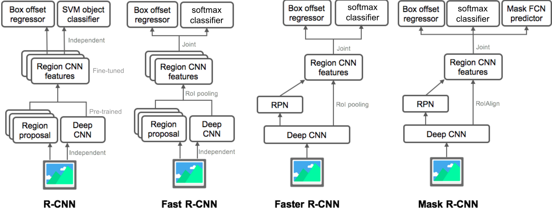
至此这系列这些东西，大概就搞明白了，当然，要是真有时间还是可以去看源码。这个图可以大概看看，有点细节不是很懂为什么这么画。

凭记忆回溯一下这几个方法的思路历程

R-CNN：selective search + warp + 类别和回归loss模式。就是使用selective search选出proposals(region proposals, region of interest, 总之就是表示我们预设的可能会出现object的有前途的region)，然后warp它们为一个fixed的大小，输入cnn，得到feature vector，并行输到classification和bbox regression。我们label/groundtruth是在图片上的各bbox的位置大小和代表的类，与我们的region通过iou来界定。classification预测这个region对于各class的confidence/probability，如果足够bbox regression也有效，注意一个regression也是针对每个class的。
- 所以，对于一开始的2000个region proposals，都要过一遍cnn，然后每个都要针对各class
- R-CNN 虽然最 vanilla但是提供了object detection这个事各种基本的设定，比如分开classification和regression的这个workflow
Fast R-CNN：selective search + 不用挨个forward + RoI Pooling. 改进了产生各proposal的vector的workflow，之前是image → selective search → proposals → warp → cnn → feature vector，现在是image → cnn → feature map, image → selective search → proposals, proposals 利用cnn结构关系映射到feature map上的proposals → roi pooling → fcfc → feature vector
- Fast R-CNN就是1. 不用每个proposal单独forward一次network了，直接forward整个image，根据映射直接索取对应的feature map 2. roi pooling取代了warp 3. classification和regression一体的loss function
Faster R-CNN：RPN + 循环式训练 + Fast R-CNN. 再次针对 selective search进行了改进。现在image → cnn → feature map, feature map → rpn → proposals（先单独train，也具有classification和bbox regression但classification只有两类，也就是判断有没有object）, feature map + feature map proposals → roi pooling → 正式的Fast R-CNN → feature vector → classification and regression
- Faster R-CNN 就是把到现在唯一剩下的不太舒服的，割裂开的生成proposals这件事也优雅地放入了网络，思路就是，直接以一个前置的先驱的类Fast R-CNN来得到有潜力的 proposals，因为可以想象，前面我们设计好的机制（e.g., classification + regression）无非就是在proposals上做文章，以其为基础，判断它是不是还真有个object以及fine-tune它的位置尺寸，那么其实去生成proposal这件事本身也就可以这样来做，基于一些“最基本的proposal”，也就是我们所设的，硬编码好的anchors们，它们以不同尺度size，locates在不同grid遍布image，等待着被筛选和fine-tune成proposals。于是也可以想象，这个时候的classification，肯定不是所有的classes了，毕竟我们还不是做最终的检测，所以不过是这个anchor，要不要成为proposal的2个
- 所以大概而言，几个主要的key points就是1. RPN (最重磅的contribution) 2. Faster R-CNN 的训练过程也很有意思，是先训RPN，然后现在能生成proposals了，就训后面的Fast R-CNN（或者说开始训Faster R-CNN），然后把后面训好的参数，和RPN shared的conv部分重新initialize，再训RPN，然后弄好之后再一次训后面的（可以发现到此次训练，两个网络shared部分是相同的）。这个过程可以想象可以一直做，不过这样的两次就可以了
- Note: 后续很值得看一下Faster R-CNN的源码，肯定是有很多细节的
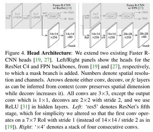
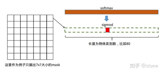
Mask R-CNN ：几个点就是1. 新加了neck的使用情况，现在可以用ResNet + FPN 2. RoI Align的设计使quantization mis-alignment 问题改进 3. 关于预测mask这个问题的设计：使用不干扰主流Faster R-CNN的方式，在head里on parallel加入预测mask的branch；mask是class-wise的，尺寸为m*m*K （e.g., 28*28*80）；计算loss时，该像素对应的ground-truth label对应的channel位置的那个binary值才计算loss；在test time像素mask的预测是根据classification的结果来的

R-CNN (Region-based CNN) (2014)#

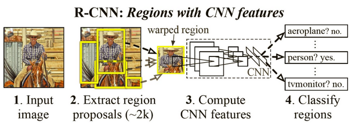
The main idea is composed of two steps. First, using selective search, it identifies a manageable number of bounding-box object region candidates (“region of interest” or “RoI”). And then it extracts CNN features from each region independently for classification
Model Workflow. How R-CNN works can be summarized as follows:
- Pre-train a CNN network on image classification tasks; for example, VGG or ResNet trained on ImageNet dataset. The classification task involves N classes.
- Propose category-independent regions of interest by selective search (~2k candidates per image). Those regions may contain target objects and they are of different sizes.
- Region candidates are warped to have a fixed size as required by CNN. (image warping is non-uniform resizing, according to the Learning OpenCV I learned earlier)
- Continue fine-tuning the CNN on warped proposal regions for K + 1 classes; The additional one class refers to the background (no object of interest). In the fine-tuning stage, we should use a much smaller learning rate and the mini-batch oversamples the positive cases because most proposed regions are just background.
- Given every image region, one forward propagation through the CNN generates a feature vector. This feature vector is then consumed by a binary SVM trained for each class independently. The positive samples are proposed regions with IoU (intersection over union) overlap threshold >= 0.3, and negative samples are irrelevant others.
- To reduce the localization errors, a regression model is trained to correct the predicted detection window on bounding box correction offset using CNN features.
Bounding Box Regression
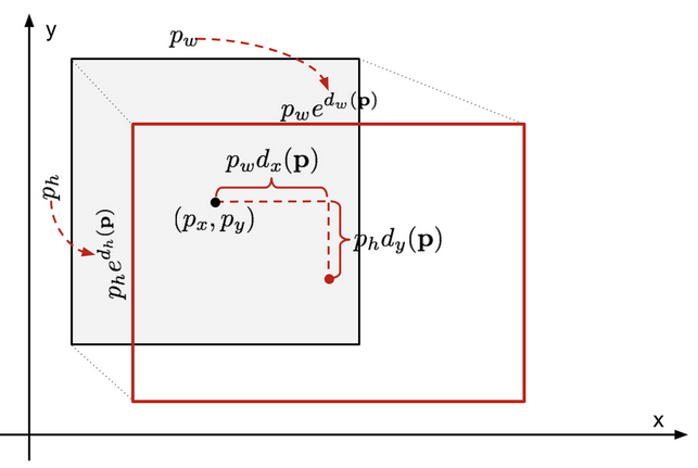
- Note: 这里的逻辑是这样的， $p = (p_{x}, p_{y}, p_{w}, p_{h})$ 是目前预测的box， $g = (g_{x}, g_{y}, g_{w}, g_{h})$ 是ground-truth box，我们现在想预测出来一个transformation去让预测的靠过去ground-truth。为了使其平移的两项scale-invariant，让放大缩小的两项log-scale，该transformation往那靠的组成方式就设计为了如下公式。
- 于是总的来说：current box vector $p = (p_{x}, p_{y}, p_{w}, p_{h})$ → regressor → offset vector $d (p) = (d_{x}, d_{y}, d_{w}, d_{h}))$ → + shape and + exp() → applied on current box → refined box vector $\hat{g} = ({\hat{g}}_{x}, {\hat{g}}_{y}, {\hat{g}}_{w}, {\hat{g}}_{h})$ ，
- 而如果就是完美的情况，也就是最后得到的是 $g = (g_{x}, g_{y}, g_{w}, g_{h})$ 时，我们能够知道反过去的 $d (p) = (d_{x}, d_{y}, d_{w}, d_{h}))$ 的值应该为 $t = (t_{x}, t_{y}, t_{w}, t_{h})$ ，这，也就正是我们想要我们这个输出offset的regressor想要输出的target。于是，最后的loss fucntion 也就是比较我们当前的作为要去往ground-truth靠的d(p)和对于它的“标签”target的L2 loss
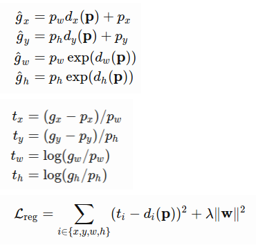
- Use 4 bounding box correction functions d_i on the whole prediction vector to approach the gt
- Not all the predicted bounding boxes have corresponding ground truth boxes. If there is no overlap, not run bbox regression. Here, only a predicted box with a nearby ground truth box with at least 0.6 IoU is kept for training the bbox regression model

个人小结：整个过程大概是这样的：1. 在image上通过selective search的策略提取约2k个regions，然后2. 通过warp使得它们有统一的大小，3. 进而输入到cnn中，每个region都可得到一个feature vector，实际上是用的AlexNet，输出了4096维的vector，然后4. 分别进入对每个类都有的自己的binary svm。另外在这里，训练的时候也就关系到了ground-truth是怎么设计的，原image上的ground-truth box在这里也就是贡献到了给binary svm 是或否的信息，对于每个proposal，对于每个其附近有iou足够（>0.5）的ground-truth，这个proposal的对于那个ground-truth所对应的class的svm的label就是个positive，也就是应该为1，大概就是这样一个逻辑。然后5. 对于有的话就计算bounding box的loss

Problem: Speed Bottleneck. Running selective search to propose 2000 region candidates for every image; Generating the CNN feature vector for every image region (N images * 2000).

Fast R-CNN (2015)#

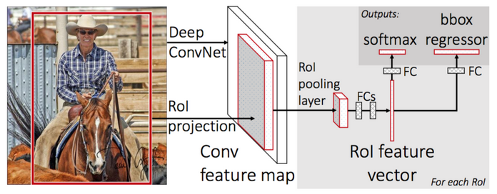
To make R-CNN faster, Girshick (2015) improved the training procedure by unifying three independent models into one jointly trained framework and increasing shared computation results, named Fast R-CNN.
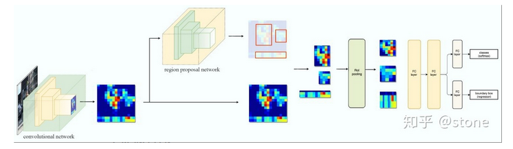
Instead of extracting CNN feature vectors independently for each region proposal, this model aggregates them into one CNN forward pass over the entire image and the region proposals share this feature matrix. Then the same feature matrix is branched out to be used for learning the object classifier and the bounding-box regressor. In conclusion, computation sharing speeds up R-CNN
Why don't we input the whole image to the cnn. At first we also have our region proposals by selective search, and since this is just a cnn, we know the projection of them on the feature map (we know the strides, ...)
In the previous, we use warping image to make patches sizes the same. here the roi pooling layer do this for us. e.g., for each proposal the outcome will be 7x7x512. and another difference from r-cnn is that there we do this warping at the beginning but here it's on the learned features
ROI pooling
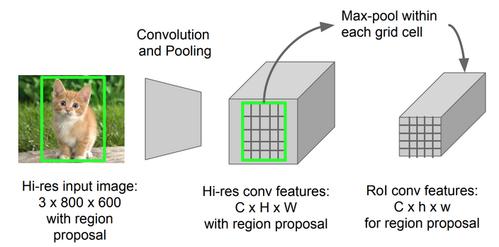
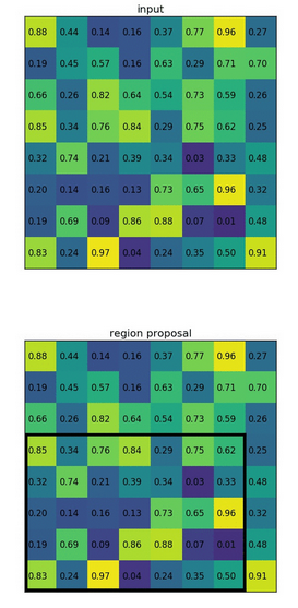
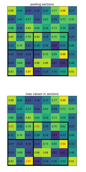
- It is a type of max pooling to convert features in the projected region of the image of any size, h x w, into a small fixed window, H x W. The input region is divided into H x W grids, approximately every subwindow of size h/H x w/W. Then apply max-pooling in each grid
- Convert the features inside any valid region of interest into a small feature map with a fixed spatial extent of H × W (e.g., 7 × 7)
- RoI max pooling works by dividing the h × w RoI window into an H × W grid of sub-windows of approximate size h/H × w/W and then max-pooling the values in each sub-window into the corresponding output grid cell
- Note: 我感觉上面这个图的H, W的表示和h, w反了，文章中H, W表示的是RoI的目标标准大小
Loss function
- The model is optimized for a loss combining two tasks (classification + localization):
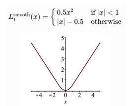
- The loss function sums up the cost of classification and bounding box prediction: L=L_cls+L_box. For “background” RoI, L_box is ignored by the indicator function 1[u≥1]:
  
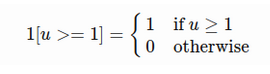
  The overall loss function is:
  
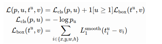
  Note: 这里的符号和之前R-CNN比有些混乱。总之，就是classification的softmax (其在文章里说的是log loss for class u)和经indicator function选定的regression的smooth L1相加
Model workflow:
- First, pre-train a convolutional neural network on image classification tasks.
- Propose regions by selective search (~2k candidates per image)
- Alter the pre-trained CNN:
  - Replace the last max pooling layer of the pre-trained CNN with a RoI pooling layer. The RoI pooling layer outputs fixed-length feature vectors of region proposals. Sharing the CNN computation makes a lot of sense, as many region proposals of the same images are highly overlapped.
  - Replace the last fully connected layer and the last softmax layer (K classes) with a fully connected layer and softmax over K + 1 classes
- Finally the model branches into two output layers:
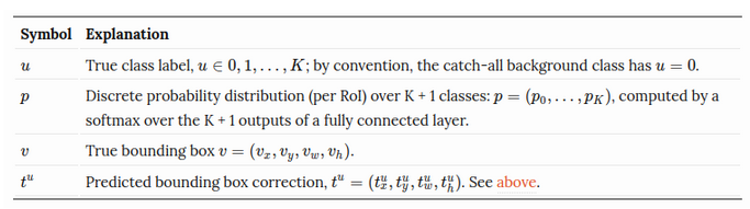
  - A softmax estimator of K + 1 classes (same as in R-CNN, +1 is the “background” class), outputting a discrete probability distribution per RoI.
  - A bounding-box regression model which predicts offsets relative to the original RoI (ground truth) for each of K classes (again, if the class in the classification is with low confidence that is under the threshold, we do not need to do the regression for this class)

Problem: Speed Bottleneck. Fast R-CNN is much faster in both training and testing time. However, the improvement is not dramatic because the region proposals are generated separately by another model and that is very expensive.

Faster R-CNN (2016)#

An intuitive speedup solution is to integrate the region proposal algorithm into the CNN model. Faster R-CNN (Ren et al., 2016) is doing exactly this: construct a single, unified model composed of RPN (region proposal network) and fast R-CNN with shared convolutional feature layers
Model Workflow:
- Pre-train a CNN network on image classification tasks.
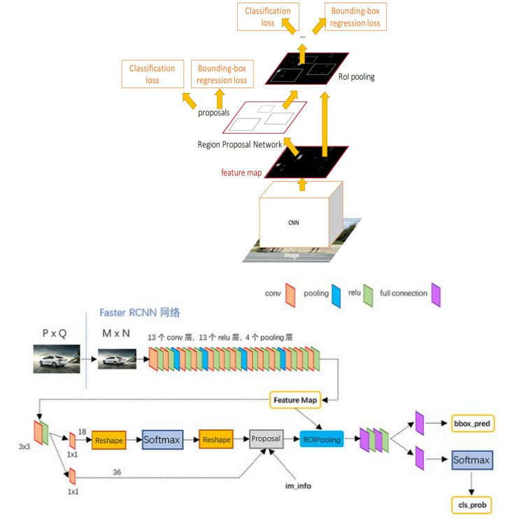
  - Note: conv层们都用kernel 3，stride 1和pad 1使得没有降采样，而pooling们都是kernel 2，0 pad和stride 2降一倍。四个pooling层使得feature map是(M/16)x(N/16)。这样的feature map和原图的对应关系会很明显。
- Fine-tune the RPN (region proposal network) end-to-end for the region proposal task, which is initialized by the pre-train image classifier. Positive samples have IoU (intersection-over-union) > 0.7, while negative samples have IoU < 0.3
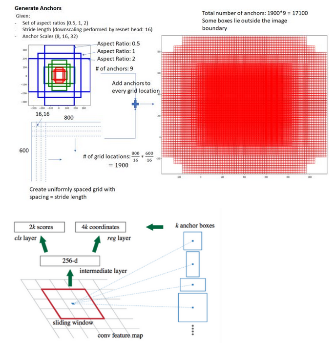
  - Slide a small n x n spatial window over the conv feature map of the entire image
  - At the center of each sliding window, we predict multiple regions of various scales and ratios simultaneously. An anchor is a combination of (sliding window center, scale, ratio). For example, 3 scales + 3 ratios => k=9 anchors at each sliding position
  - Note: 其实anchor不是什么继续传递下去的output，就是一些“设定”，表示我们用的regions们。在前面的cnn输出feature map后得到HxWxC，这里的C可能很大。再用一层3x3变为HxWx256，所以一个像素点就是深度下去的一个256维向量，此时选取anchors（个人认为：其实是对于image设定anchors，不过会参考feature map的尺寸降维情况，使得每个anchor对应于最后feature map上的每个pixel，才使得label有意义，所以相当于把这个anchor的任务自然分配到了最后feature map上的每个pixel以及其channels上）。通常anchors在尺度和尺寸上各有三种选择，综合下来就是9种搭配，也就是k=9，也就是对于sliding window中每个像素点对应的256维向量，我们为它设定了9个区域
  - 然后一层1x1的conv作为一个二分类器，对该256维向量相关的9个区域中是否有object进行判断，于是对于该点产生2k个score(2*k, here k=9)(也就是channels数量)。另外还有平行的一层1x1目标为bounding box regression，于是是4k个channels
  - 注意在这里的classfication只有有无object，而最终的那个分类是有确定的label
  - Note: 另外在anchor具体是怎么应用的这个事上，个人是这样感觉的，其不会像真正的proposals一样在feature map上crop出来roi pooling之类的，而是体现在训练RPN这个地方label的制作上，可以想象目标值自然是需要ground-truth和anchor的信息对应着来的。而且，看最上面第二个图也可以发现，这里不过就是用conv得到了channels是18 (9x2)和36 (9x4)的输出而已，然后就用这个vector算loss了，所以肯定是自然而然地蕴涵在我们让这些元素去的位置上了
- Train a Fast R-CNN object detection model using the proposals generated by the current RPN
- Then again, reversely, use the Fast R-CNN network to initialize RPN training. While keeping the shared convolutional layers, only fine-tune the RPN-specific layers. At this stage, RPN and the detection network have shared convolutional layers!
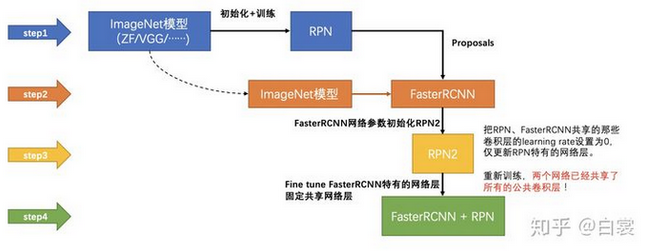
- Finally fine-tune the unique layers of Fast R-CNN
- Step 4-5 can be repeated to train RPN and Fast R-CNN alternatively if needed. But "A similar alternating training can be run for more iterations, but we have observed negligible improvements”. Twice for now is pretty enough
Loss function
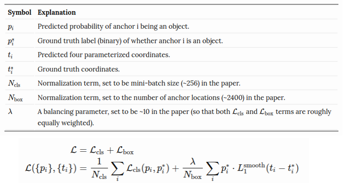
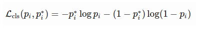
- Note: 这里说的是RPN的训练，同样，softmax + smooth L1。当然可以想象和最终的那个loss一样设计，区别不过是在这里只有两类所以是

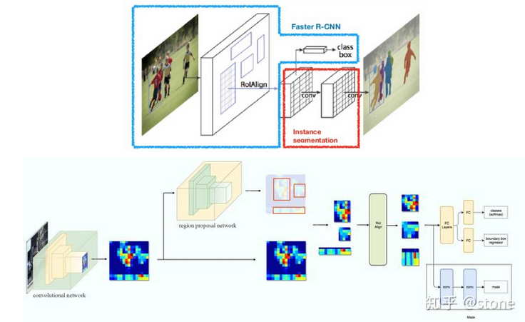
Mask R-CNN (2017)#

Mask R-CNN (He et al., 2017) extends Faster R-CNN to pixel-level image segmentation. Mask R-CNN is conceptually simple: Faster R-CNN has two outputs for each candidate object, a class label and a bounding-box offset; to this we add a third branch that outputs the object mask.

记录：PyTorch中之前自己拿来用过的模型

MaskRCNN(
  (transform): GeneralizedRCNNTransform(
      Normalize(mean=[0.485, 0.456, 0.406], std=[0.229, 0.224, 0.225])
      Resize(min_size=(800,), max_size=1333, mode='bilinear')
  )
  (backbone): BackboneWithFPN(
    (body): IntermediateLayerGetter(
      (conv1): Conv2d(3, 64, kernel_size=(7, 7), stride=(2, 2), padding=(3, 3), bias=False)
      (bn1): FrozenBatchNorm2d(64)
      (relu): ReLU(inplace=True)
      (maxpool): MaxPool2d(kernel_size=3, stride=2, padding=1, dilation=1, ceil_mode=False)
      (layer1): Sequential(
        (0): Bottleneck(
          (conv1): Conv2d(64, 64, kernel_size=(1, 1), stride=(1, 1), bias=False)
          (bn1): FrozenBatchNorm2d(64)
          (conv2): Conv2d(64, 64, kernel_size=(3, 3), stride=(1, 1), padding=(1, 1), bias=False)
          (bn2): FrozenBatchNorm2d(64)
          (conv3): Conv2d(64, 256, kernel_size=(1, 1), stride=(1, 1), bias=False)
          (bn3): FrozenBatchNorm2d(256)
          (relu): ReLU(inplace=True)
          (downsample): Sequential(
            (0): Conv2d(64, 256, kernel_size=(1, 1), stride=(1, 1), bias=False)
            (1): FrozenBatchNorm2d(256)
          )
        )
        (1): Bottleneck(
          (conv1): Conv2d(256, 64, kernel_size=(1, 1), stride=(1, 1), bias=False)
          (bn1): FrozenBatchNorm2d(64)
          (conv2): Conv2d(64, 64, kernel_size=(3, 3), stride=(1, 1), padding=(1, 1), bias=False)
          (bn2): FrozenBatchNorm2d(64)
          (conv3): Conv2d(64, 256, kernel_size=(1, 1), stride=(1, 1), bias=False)
          (bn3): FrozenBatchNorm2d(256)
          (relu): ReLU(inplace=True)
        )
        (2): Bottleneck(
          (conv1): Conv2d(256, 64, kernel_size=(1, 1), stride=(1, 1), bias=False)
          (bn1): FrozenBatchNorm2d(64)
          (conv2): Conv2d(64, 64, kernel_size=(3, 3), stride=(1, 1), padding=(1, 1), bias=False)
          (bn2): FrozenBatchNorm2d(64)
          (conv3): Conv2d(64, 256, kernel_size=(1, 1), stride=(1, 1), bias=False)
          (bn3): FrozenBatchNorm2d(256)
          (relu): ReLU(inplace=True)
        )
      )
      (layer2): Sequential(
        (0): Bottleneck(
          (conv1): Conv2d(256, 128, kernel_size=(1, 1), stride=(1, 1), bias=False)
          (bn1): FrozenBatchNorm2d(128)
          (conv2): Conv2d(128, 128, kernel_size=(3, 3), stride=(2, 2), padding=(1, 1), bias=False)
          (bn2): FrozenBatchNorm2d(128)
          (conv3): Conv2d(128, 512, kernel_size=(1, 1), stride=(1, 1), bias=False)
          (bn3): FrozenBatchNorm2d(512)
          (relu): ReLU(inplace=True)
          (downsample): Sequential(
            (0): Conv2d(256, 512, kernel_size=(1, 1), stride=(2, 2), bias=False)
            (1): FrozenBatchNorm2d(512)
          )
        )
        (1): Bottleneck(
          (conv1): Conv2d(512, 128, kernel_size=(1, 1), stride=(1, 1), bias=False)
          (bn1): FrozenBatchNorm2d(128)
          (conv2): Conv2d(128, 128, kernel_size=(3, 3), stride=(1, 1), padding=(1, 1), bias=False)
          (bn2): FrozenBatchNorm2d(128)
          (conv3): Conv2d(128, 512, kernel_size=(1, 1), stride=(1, 1), bias=False)
          (bn3): FrozenBatchNorm2d(512)
          (relu): ReLU(inplace=True)
        )
        (2): Bottleneck(
          (conv1): Conv2d(512, 128, kernel_size=(1, 1), stride=(1, 1), bias=False)
          (bn1): FrozenBatchNorm2d(128)
          (conv2): Conv2d(128, 128, kernel_size=(3, 3), stride=(1, 1), padding=(1, 1), bias=False)
          (bn2): FrozenBatchNorm2d(128)
          (conv3): Conv2d(128, 512, kernel_size=(1, 1), stride=(1, 1), bias=False)
          (bn3): FrozenBatchNorm2d(512)
          (relu): ReLU(inplace=True)
        )
        (3): Bottleneck(
          (conv1): Conv2d(512, 128, kernel_size=(1, 1), stride=(1, 1), bias=False)
          (bn1): FrozenBatchNorm2d(128)
          (conv2): Conv2d(128, 128, kernel_size=(3, 3), stride=(1, 1), padding=(1, 1), bias=False)
          (bn2): FrozenBatchNorm2d(128)
          (conv3): Conv2d(128, 512, kernel_size=(1, 1), stride=(1, 1), bias=False)
          (bn3): FrozenBatchNorm2d(512)
          (relu): ReLU(inplace=True)
        )
      )
      (layer3): Sequential(
        (0): Bottleneck(
          (conv1): Conv2d(512, 256, kernel_size=(1, 1), stride=(1, 1), bias=False)
          (bn1): FrozenBatchNorm2d(256)
          (conv2): Conv2d(256, 256, kernel_size=(3, 3), stride=(2, 2), padding=(1, 1), bias=False)
          (bn2): FrozenBatchNorm2d(256)
          (conv3): Conv2d(256, 1024, kernel_size=(1, 1), stride=(1, 1), bias=False)
          (bn3): FrozenBatchNorm2d(1024)
          (relu): ReLU(inplace=True)
          (downsample): Sequential(
            (0): Conv2d(512, 1024, kernel_size=(1, 1), stride=(2, 2), bias=False)
            (1): FrozenBatchNorm2d(1024)
          )
        )
        (1): Bottleneck(
          (conv1): Conv2d(1024, 256, kernel_size=(1, 1), stride=(1, 1), bias=False)
          (bn1): FrozenBatchNorm2d(256)
          (conv2): Conv2d(256, 256, kernel_size=(3, 3), stride=(1, 1), padding=(1, 1), bias=False)
          (bn2): FrozenBatchNorm2d(256)
          (conv3): Conv2d(256, 1024, kernel_size=(1, 1), stride=(1, 1), bias=False)
          (bn3): FrozenBatchNorm2d(1024)
          (relu): ReLU(inplace=True)
        )
        (2): Bottleneck(
          (conv1): Conv2d(1024, 256, kernel_size=(1, 1), stride=(1, 1), bias=False)
          (bn1): FrozenBatchNorm2d(256)
          (conv2): Conv2d(256, 256, kernel_size=(3, 3), stride=(1, 1), padding=(1, 1), bias=False)
          (bn2): FrozenBatchNorm2d(256)
          (conv3): Conv2d(256, 1024, kernel_size=(1, 1), stride=(1, 1), bias=False)
          (bn3): FrozenBatchNorm2d(1024)
          (relu): ReLU(inplace=True)
        )
        (3): Bottleneck(
          (conv1): Conv2d(1024, 256, kernel_size=(1, 1), stride=(1, 1), bias=False)
          (bn1): FrozenBatchNorm2d(256)
          (conv2): Conv2d(256, 256, kernel_size=(3, 3), stride=(1, 1), padding=(1, 1), bias=False)
          (bn2): FrozenBatchNorm2d(256)
          (conv3): Conv2d(256, 1024, kernel_size=(1, 1), stride=(1, 1), bias=False)
          (bn3): FrozenBatchNorm2d(1024)
          (relu): ReLU(inplace=True)
        )
        (4): Bottleneck(
          (conv1): Conv2d(1024, 256, kernel_size=(1, 1), stride=(1, 1), bias=False)
          (bn1): FrozenBatchNorm2d(256)
          (conv2): Conv2d(256, 256, kernel_size=(3, 3), stride=(1, 1), padding=(1, 1), bias=False)
          (bn2): FrozenBatchNorm2d(256)
          (conv3): Conv2d(256, 1024, kernel_size=(1, 1), stride=(1, 1), bias=False)
          (bn3): FrozenBatchNorm2d(1024)
          (relu): ReLU(inplace=True)
        )
        (5): Bottleneck(
          (conv1): Conv2d(1024, 256, kernel_size=(1, 1), stride=(1, 1), bias=False)
          (bn1): FrozenBatchNorm2d(256)
          (conv2): Conv2d(256, 256, kernel_size=(3, 3), stride=(1, 1), padding=(1, 1), bias=False)
          (bn2): FrozenBatchNorm2d(256)
          (conv3): Conv2d(256, 1024, kernel_size=(1, 1), stride=(1, 1), bias=False)
          (bn3): FrozenBatchNorm2d(1024)
          (relu): ReLU(inplace=True)
        )
      )
      (layer4): Sequential(
        (0): Bottleneck(
          (conv1): Conv2d(1024, 512, kernel_size=(1, 1), stride=(1, 1), bias=False)
          (bn1): FrozenBatchNorm2d(512)
          (conv2): Conv2d(512, 512, kernel_size=(3, 3), stride=(2, 2), padding=(1, 1), bias=False)
          (bn2): FrozenBatchNorm2d(512)
          (conv3): Conv2d(512, 2048, kernel_size=(1, 1), stride=(1, 1), bias=False)
          (bn3): FrozenBatchNorm2d(2048)
          (relu): ReLU(inplace=True)
          (downsample): Sequential(
            (0): Conv2d(1024, 2048, kernel_size=(1, 1), stride=(2, 2), bias=False)
            (1): FrozenBatchNorm2d(2048)
          )
        )
        (1): Bottleneck(
          (conv1): Conv2d(2048, 512, kernel_size=(1, 1), stride=(1, 1), bias=False)
          (bn1): FrozenBatchNorm2d(512)
          (conv2): Conv2d(512, 512, kernel_size=(3, 3), stride=(1, 1), padding=(1, 1), bias=False)
          (bn2): FrozenBatchNorm2d(512)
          (conv3): Conv2d(512, 2048, kernel_size=(1, 1), stride=(1, 1), bias=False)
          (bn3): FrozenBatchNorm2d(2048)
          (relu): ReLU(inplace=True)
        )
        (2): Bottleneck(
          (conv1): Conv2d(2048, 512, kernel_size=(1, 1), stride=(1, 1), bias=False)
          (bn1): FrozenBatchNorm2d(512)
          (conv2): Conv2d(512, 512, kernel_size=(3, 3), stride=(1, 1), padding=(1, 1), bias=False)
          (bn2): FrozenBatchNorm2d(512)
          (conv3): Conv2d(512, 2048, kernel_size=(1, 1), stride=(1, 1), bias=False)
          (bn3): FrozenBatchNorm2d(2048)
          (relu): ReLU(inplace=True)
        )
      )
    )
    (fpn): FeaturePyramidNetwork(
      (inner_blocks): ModuleList(
        (0): Conv2d(256, 256, kernel_size=(1, 1), stride=(1, 1))
        (1): Conv2d(512, 256, kernel_size=(1, 1), stride=(1, 1))
        (2): Conv2d(1024, 256, kernel_size=(1, 1), stride=(1, 1))
        (3): Conv2d(2048, 256, kernel_size=(1, 1), stride=(1, 1))
      )
      (layer_blocks): ModuleList(
        (0): Conv2d(256, 256, kernel_size=(3, 3), stride=(1, 1), padding=(1, 1))
        (1): Conv2d(256, 256, kernel_size=(3, 3), stride=(1, 1), padding=(1, 1))
        (2): Conv2d(256, 256, kernel_size=(3, 3), stride=(1, 1), padding=(1, 1))
        (3): Conv2d(256, 256, kernel_size=(3, 3), stride=(1, 1), padding=(1, 1))
      )
      (extra_blocks): LastLevelMaxPool()
    )
  )
  (rpn): RegionProposalNetwork(
    (anchor_generator): AnchorGenerator()
    (head): RPNHead(
      (conv): Conv2d(256, 256, kernel_size=(3, 3), stride=(1, 1), padding=(1, 1))
      (cls_logits): Conv2d(256, 3, kernel_size=(1, 1), stride=(1, 1))
      (bbox_pred): Conv2d(256, 12, kernel_size=(1, 1), stride=(1, 1))
    )
  )
  (roi_heads): RoIHeads(
    (box_roi_pool): MultiScaleRoIAlign()
    (box_head): TwoMLPHead(
      (fc6): Linear(in_features=12544, out_features=1024, bias=True)
      (fc7): Linear(in_features=1024, out_features=1024, bias=True)
    )
    (box_predictor): FastRCNNPredictor(
      (cls_score): Linear(in_features=1024, out_features=2, bias=True)
      (bbox_pred): Linear(in_features=1024, out_features=8, bias=True)
    )
    (mask_roi_pool): MultiScaleRoIAlign()
    (mask_head): MaskRCNNHeads(
      (mask_fcn1): Conv2d(256, 256, kernel_size=(3, 3), stride=(1, 1), padding=(1, 1))
      (relu1): ReLU(inplace=True)
      (mask_fcn2): Conv2d(256, 256, kernel_size=(3, 3), stride=(1, 1), padding=(1, 1))
      (relu2): ReLU(inplace=True)
      (mask_fcn3): Conv2d(256, 256, kernel_size=(3, 3), stride=(1, 1), padding=(1, 1))
      (relu3): ReLU(inplace=True)
      (mask_fcn4): Conv2d(256, 256, kernel_size=(3, 3), stride=(1, 1), padding=(1, 1))
      (relu4): ReLU(inplace=True)
    )
    (mask_predictor): MaskRCNNPredictor(
      (conv5_mask): ConvTranspose2d(256, 256, kernel_size=(2, 2), stride=(2, 2))
      (relu): ReLU(inplace=True)
      (mask_fcn_logits): Conv2d(256, 2, kernel_size=(1, 1), stride=(1, 1))
    )
  )
)

(Optionally) use ResNet-FPN (upgrade Faster R-CNN by FPN)
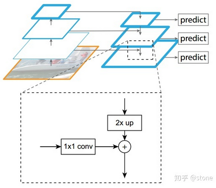
- Feature Pyramid Network (FPN): 自下而上，自上而下和横向连接，为多尺度检测设计
- 将ResNet-FPN和Fast R-CNN 进行结合，实际上就是Faster R-CNN 的了，但与最初的Faster R-CNN不同的是，FPN 产生了特征金字塔，而并非只是一个feature map。个人感觉之后是用FPN得到的最终的那一个map给RPN，然后去fine-tune proposals们（反映在所output的channels里），就得到了image上fine-tune好的RoI们，然后再用定好的一个公式决定往下映射到第几层的map去crop出要输给RoI pooling / RoI align / warp的feature patch。其效果就是：大尺度的ROI从低分辨率（更底层，尺寸更小channels可更深的）的feature map上切，有利于检测大目标，小尺度的ROI要从高分辨率的（更上面的）feature map上切，有利于检测小目标
RoI Align to replace RoI pooling
- RoIPool [12] is a standard operation for extracting a small feature map (e.g., 7×7) from each RoI. [...]. Quantization is performed, e.g., on a continuous coordinate x by computing [x/16], where 16 is a feature map stride and [·] is rounding; likewise, quantization is performed when dividing into bins (e.g., 7×7)
- These quantizations introduce mis-alignments between the RoI and the extracted features. (因为一开始image的RoI和后面映射过去的feature map上对应的patch不是完美对应的) While this may not impact classification, which is robust to small translations, it has a large negative effect on predicting pixel-accurate masks.
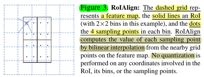
- Our proposed change is simple: we avoid any quantization of the RoI boundaries or bins (i.e., we use x/16 instead of [x/16]). We use bilinear interpolation [22] to compute the exact values of the input features at four regularly sampled locations in each RoI bin, and aggregate the result (using max or average)
- Note: 个人总结也就是，之前为了得到对应的映射，总是需要quantization，体现在1. 从RoI到feature map上的RoI映射时：[x/16]，因为这样才能到feature map上存在的grid点上，然后2. 为了得到统一尺寸划分feature map上的RoI的格子时，没法等分，比如2x2的上面一半比下面少一行这样的情况，也属于quantization，产生了mis-alignment；于是在这里，所有的操作我都不quantization，具体就是我1. x/16而且2. 直接划（可以从图上看出来，solid lines就是完美的这个应该在的位置，而且格子也是完美划的），然后对于每个划好的grid，能够确定它们的值就行了。采取的策略就是每个值的grid内取4个sampling point（数字4是作者测出来效果较好的），然后取它们的值的pool即可。当然，这4个点显然不会在格子上，很显然可以用bilinear interpolation轻松解决（这其实也就是最后我们这整个RoI Align把问题归结到这个具体的事情上，用插值把gap填补好了）
Loss Function
- The multi-task loss function of Mask R-CNN combines the loss of classification, localization and segmentation mask: L=L_cls+L_box+L_mask, where L_cls and L_box are same as in Faster R-CNN
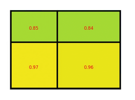
- The mask branch generates a mask of dimension m x m for each RoI and each class; K classes in total. Thus, the total output is of size K⋅m^2. Because the model is trying to learn a mask for each class, there is no competition among classes for generating masks
- L_mask is defined as the average binary cross-entropy loss, only including k-th mask if the region is associated with the ground truth class k
  
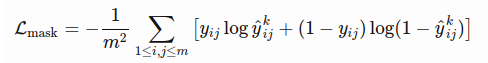
  where $y_{i j}$ is the label of a cell (i, j) in the true mask for the region of size m x m; $y_{i j}^{k}$ is the predicted value of the same cell in the mask learned for the ground-truth class k
- Note: 假设一共有K个类别，则mask分割分支的输出维度是 mmK, 对于 m*m 中的每个点，都会输出K个二值Mask（每个类别使用sigmoid输出）。需要注意的是，计算loss的时候，并不是每个类别的sigmoid输出都计算二值交叉熵损失，而是该像素属于哪个类，哪个类的sigmoid输出才要计算损失(如图红色方形所示)。并且在测试的时候，我们是通过分类分支预测的类别来选择相应的mask预测。这样，mask预测和分类预测就彻底解耦了