第二章微分方程与差分方程模型

2.1 常微分方程的求解

2.1.1 符号解求解

例1（符号解）

$y^{\prime \prime}+2 y^{\prime}+y=x^{2}$

from sympy import *

y = symbols('y', cls=Function)
x = symbols('x')
eq = Eq(y(x).diff(x,2)+2*y(x).diff(x,1)+y(x),x*x)
print(dsolve(eq,y(x)))

输出：
Eq(y(x), x**2 - 4*x + (C1 + C2*x)*exp(-x) + 6)

例2（符号解）

$\left\{\begin{array}{l}y^{\prime \prime}+4 y^{\prime}+29 y=0 \\ y(0)=0, y^{\prime}(0)=15\end{array}\right.$

y = symbols('y',cls = Function)
x = symbols('x')
eq = Eq(y(x).diff(x,2)+4*y(x).diff(x,1)+29*y(x),0)
print(dsolve(eq,y(x)))

C1 = symbols('C1')
C2 = symbols('C2')
f = (C1*sin(5*x) + C2*cos(5*x)) * exp(-2*x)
print(f.diff(x,1))

输出：
Eq(y(x), (C1*sin(5*x) + C2*cos(5*x))*exp(-2*x))
-2*(C1*sin(5*x) + C2*cos(5*x))*exp(-2*x) + (5*C1*cos(5*x) - 5*C2*sin(5*x))*exp(-2*x)

2.1.2 数值解求解

本质上内部ode使用到了欧拉法和龙格库塔法

例1

$y^{\prime}=x^{2}+y^{2}$

from scipy.integrate import odeint
from numpy import arange

dy = lambda y,x: x**2+y**2
x = arange(0,10.5,0.5)
sol = odeint(dy,0,x)
print("x={}\n对应的数值解y={}".format(x,sol.T))

输出：
x=[ 0.   0.5  1.   1.5  2.   2.5  3.   3.5  4.   4.5  5.   5.5  6.   6.5
  7.   7.5  8.   8.5  9.   9.5 10. ]
对应的数值解y=[[0.00000000e+000 4.17912909e-002 3.50232067e-001 1.51744848e+000
  3.17753007e+002 4.61705896e+011 1.37961302e-306 1.05699242e-307
  8.01097889e-307 1.78020169e-306 7.56601165e-307 1.02359984e-306
  1.69118108e-306 2.22522597e-306 1.33511969e-306 1.33511018e-306
  6.89804133e-307 1.11261162e-306 8.34443015e-308 3.91792476e-317
  2.18565567e-312]]

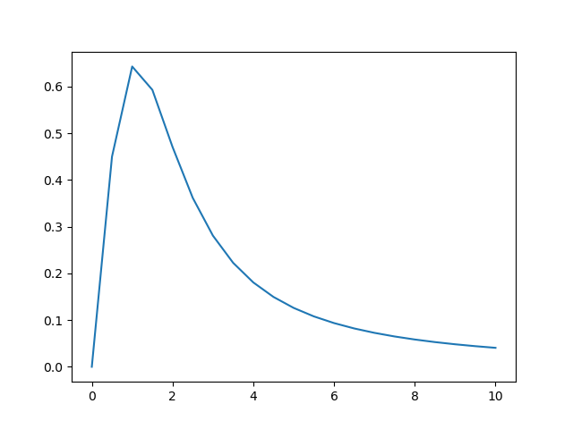
例2

$y^{\prime}=\frac{1}{x^{2}+1}-2 y^{2}, y(0)=0$

import matplotlib.pyplot as plt

dy  = lambda y,x:1/(1+x**2)-x*y**2
x = arange(0,10.5,0.5)
sol = odeint(dy,0,x)
print("x={}\n对应的数值解y={}".format(x,sol.T))
plt.plot(x,sol)
plt.show()

输出：
x=[ 0.   0.5  1.   1.5  2.   2.5  3.   3.5  4.   4.5  5.   5.5  6.   6.5
  7.   7.5  8.   8.5  9.   9.5 10. ]
对应的数值解y=[[0.         0.45001281 0.64308473 0.59306028 0.47073468 0.36183003
  0.28086488 0.2227396  0.1806778  0.14960431 0.12610963 0.10794596
  0.09361754 0.08211012 0.07272093 0.06495247 0.05844527 0.05293465
  0.04822232 0.04415738 0.04062331]]

2.1.3 高阶微分方程求解

高阶常微分方程，必须做变量替换，化为一阶微分方程组，再用odeint求数值解。

形式如下：

def f(t,y):
	'''
	要把y看作一个向量，y = [dy0,dy1,dy2,...]分别表示y的n阶导，那么y[0]就是需要求解的函数，y[1]表示一阶导，y[2]表示二阶导，以此类推
	'''
    dy1 = y[1] 		# y[1]=dy/dt,一阶导
    dy2 = -4*y[1] - 5*y[0]
    # y[0]是最初始，也就是需要求解的函数
    # 注意返回的顺序为[一阶导，二阶导]，这就形成了一阶微分方程组
    return [dy1,dy2]

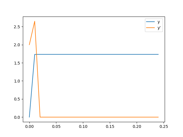
例1

$\left\{\begin{array}{l}y^{\prime \prime}-1000\left(1-y^{2}\right) y^{\prime}+y=0 \\ y(0)=0, y^{\prime}(0)=2\end{array}\right.$

import numpy as np

def fvdp(t,y):
    dy1 = y[1]
    dy2 = 1000 * (1-y[0]**2)*y[1] - y[0]
    return [dy1,dy2]

def solve_second_order_ode():
    x = arange(0,0.25,0.01)     # 给x规定范围
    y0 = [0.0,2.0]      # 初值条件
    # 初值[3.0,5.0]表示y(0) = 3,y'(0) = 5
    # 返回y，其中y[:,0]是y[0]的值，就是最终解,y[:,1]是y'(x)的值
    y = odeint(fvdp,y0,x,tfirst=True)

    y1, = plt.plot(x,y[:,0],label = 'y')
    y1_1, = plt.plot(x,y[:,1],label = 'y'')
    plt.legend(handles = [y1,y1_1])
    plt.show()

solve_second_order_ode()

输出：
x=[ 0.   0.5  1.   1.5  2.   2.5  3.   3.5  4.   4.5  5.   5.5  6.   6.5
  7.   7.5  8.   8.5  9.   9.5 10. ]
对应的数值解y=[[0.         0.45001281 0.64308473 0.59306028 0.47073468 0.36183003
  0.28086488 0.2227396  0.1806778  0.14960431 0.12610963 0.10794596
  0.09361754 0.08211012 0.07272093 0.06495247 0.05844527 0.05293465
  0.04822232 0.04415738 0.04062331]]

2.2 偏微分方程的求解

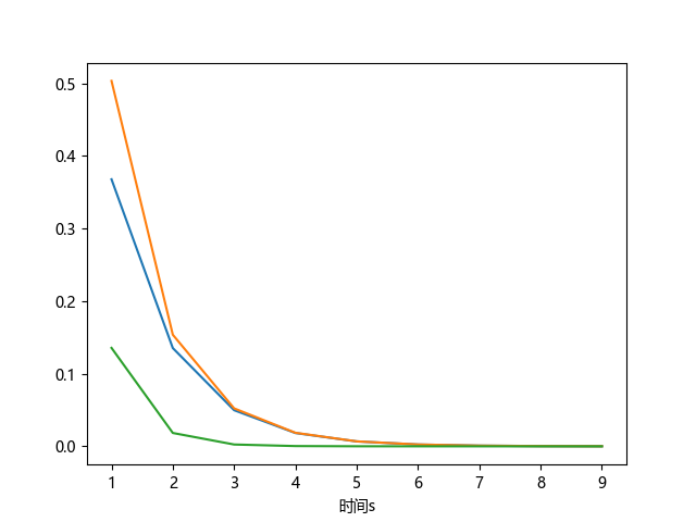
2.2.1 例1

$\left\{\begin{array}{l}\frac{d x}{d t}=2 x-3 y+3 z \\ \frac{d y}{d t}=4 x-5 y+3 z \\ \frac{d z}{d t}=4 x-4 y+2 z \\ x(0)=1, y(0)=2, z(0)=1\end{array}\right.$

import  matplotlib.pyplot as plt
from scipy.integrate import solve_ivp
import numpy as np
plt.rcParams['font.sans-serif'] = ['Microsoft YaHei']

def fun(t,w):
    x = w[0]
    y = w[1]
    z = w[2]
    return  [2*x-3*y+3*z,4*x-5*y+3*z,4*x-4*y+2*z]

# 初始条件
y0 = [1,2,1]

yy = solve_ivp(fun,(0,10),y0,method='RK45',t_eval = np.arange(1,10,1))
t = yy.t
data = yy.y
plt.plot(t,data[0,:])
plt.plot(t,data[1,:])
plt.plot(t,data[2,:]) # data[x,:]用于对图像中的线进行编号
plt.xlabel("时间s")
plt.show()

# 黄色是x 蓝色是y 绿色是z

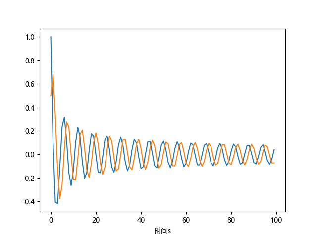
2.2.2 例2

$\left\{\begin{array}{l} \frac{d x}{d t}=-x^{3}-y \\ \frac{d y}{d t}=-y^{3}+x \\ x(0)=1, y(0)=0.5 \end{array}\right.$

def fun(t,w):
    x = w[0]
    y = w[1]
    return [-x**3-y,-y**3+x]
y0 = [1,0.5]
yy = solve_ivp(fun,(0,100),y0,method='RK45',t_eval=np.arange(0,100,1))
t = yy.t
data = yy.y
plt.plot(t,data[0,:])
plt.plot(t,data[1,:])
plt.xlabel("时间s")
plt.show()

2.3 微分方程案例

2.3.1 人口增长模型

在模型中我们假设：

不考虑死亡率对人口的影响，我们只考虑净增长率
不考虑人口迁移对问题的影响，只考虑自然变化
不考虑重大突发事件对人口的突变性影响
不考虑人口增长率变化的时滞性因素

人口增长主要用三种模型描述：
Malthus Model
Logisitc Model
Leslie Model

Malthus Model

原理

马尔萨斯模型假设增长率永远是个常数r，那么一段时间内增长个体有 $x(t+\Delta t)-x(t)=x(t) \cdot r \Delta t$

按照微分方程的形式整理：

$\left\{\begin{array}{l} \frac{d x}{d t}=x r \\ x(0)=x_{0} \end{array}\right.$

最终解得：

$x(t)=x_{0} e^{r t}$

局限性

Malthus过程呈现一个指数增长，不会发生减缓过程

Logisitc Model

原理

现在对模型进行一些修正，假设增长率会随着种群数量增加而衰减，种群最大的一个平衡数量叫K,那么可以得到:

$\left\{\begin{array}{l} \frac{d x}{d t}=x r_{\circ}\left(1-\frac{x}{K}\right) \\ x(0)=x_{0} \end{array}\right.$

解得： $x(t)=\frac{K}{1+\left(\frac{K}{x_{0}}-1\right) e^{-r t}}$

应用场景

美国人口预报

2.3.2 放射问题

放射性物质半衰期的确定建模其实非常类似于Malthus模型，因为衰变的方程可以写作:

$\left\{\begin{array}{l} \frac{d N}{d t}=-\lambda N \\ N\left(t_{0}\right)=N_{0} \end{array}\right.$

易解： $N(t)=N_{0} e^{-\lambda\left(t-t_{0}\right)}$

2.3.3 新冠传播模型

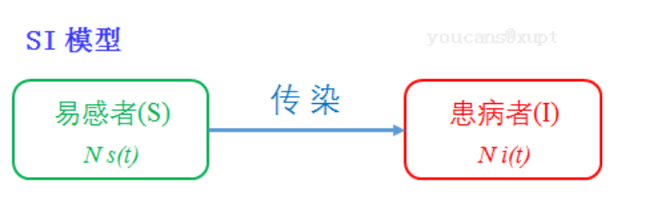
SI模型

SI模型是最简单的传染病传播模型，把人群分为易感者(S类)和患病者(I 类)两类,通过SI模型可以预测传染病高潮的到来;提高卫生水平、强化防控手段,降低病人的日接触率，可以推迟传染病高潮的到来。

原理：易感者与患病者有效接触即被感染,变为患病者,无潜伏期、无治愈情况、无免疫力。以一天作为模型的最小时间单元。总人数为N,不考虑人口的出生与死亡，迁入与迁出，此总人数不变。t时刻两类人群占总人数的比率分别记为s(t)、i(), 两类人群的数量为S(t)、l()。初始时刻t=0时，各类人数量所占初始比率为s0、i0。每个患病者每天有效接触的易感者的平均人数是λ，即日接触数。

$\mathrm{N} \frac{\mathrm{di}}{\mathrm{dt}}=\mathrm{N} \lambda \mathrm{si}$

$s(t)+i(t)=1$

解得

$\mathrm{i}(\mathrm{t})=\frac{1}{1+\left(1 / \mathrm{i}_{0}-1\right) \mathrm{e}^{-\lambda \mathrm{t}}}$

$\mathrm{I}(\mathrm{t})=\mathrm{Ni}(\mathrm{t})$

from scipy.integrate import odeint
import numpy as np
import matplotlib.pyplot as plt

def di_dt(i,t,lamda,mu):
    di_dt = lamda*i*(1-i)
    return di_dt

number = 1e7    # 总人数
lamda = 1.0     # 日接触率λ，患病者每天接触的易感者的平均人数
mu1 = 0.5       # 日治愈率N，每天被治愈的患病者人数占患病者总数的比例
i0 =1e-6   # 患病者比例的初值
tEnd = 50       # 预测日期长度
t = np.arange(0.0,tEnd,1)

yAmaly = 1/(1+(1/i0-1))*np.exp(-lamda*t)    # 运用 Logistic 模型解得的 SI 模型符号（解析）解
yInteg = odeint(di_dt,i0,t,args=(lamda,mu1))    # 求解微分方程初值问题（近似解）
yDeriv = lamda * yInteg *(1-yInteg)

# 绘图
plt.plot(t,yAmaly,'-ob',label='analytic')
plt.plot(t,yInteg,":r",label='numerical')
plt.plot(t,yDeriv,"-g",label='di_dt')
plt.title("Cpmparison between analytic and numerical solutions")
plt.legend(loc="right")
plt.axis([0,50,-0.1,1.1])
plt.show()

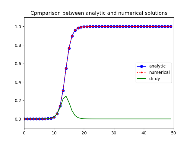
图中的红色为odeint()得到的数值解，解析解为蓝色线条，我们可以很明显的看出解析解和数值解差异很小，说明数值解的误差很小。

SIS模型

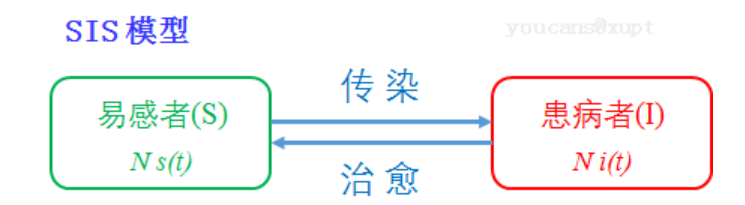
SIS 模型将人群分为 S 类和 I 类，考虑患病者（I 类）可以治愈而变成易感者（S 类），但不考虑免疫期，因此患病者（I 类）治愈变成易感者以后还可以被感染而变成患病者。

# 1. SIS 模型，常微分方程，解析解与数值解的比较
from scipy.integrate import odeint  # 导入 scipy.integrate 模块
import numpy as np  # 导入 numpy包
import matplotlib.pyplot as plt  # 导入 matplotlib包

def dy_dt(y, t, lamda, mu):  # SIS 模型，导数函数
    dy_dt = lamda*y*(1-y) - mu*y  # di/dt = lamda*i*(1-i)-mu*i
    return dy_dt

# 设置模型参数
number = 1e5  # 总人数
lamda = 1.2  # 日接触率, 患病者每天有效接触的易感者的平均人数
sigma = 2.5  # 传染期接触数
mu = lamda/sigma  # 日治愈率, 每天被治愈的患病者人数占患病者总数的比例
fsig = 1-1/sigma
y0 = i0 = 1e-5  # 患病者比例的初值
tEnd = 50  # 预测日期长度
t = np.arange(0.0,tEnd,1)  # (start,stop,step)
print("lamda={}\tmu={}\tsigma={}\t(1-1/sig)={}".format(lamda,mu,sigma,fsig))

# 解析解
if lamda == mu:
    yAnaly = 1.0/(lamda*t +1.0/i0)
else:
    yAnaly= 1.0/((lamda/(lamda-mu)) + ((1/i0)-(lamda/(lamda-mu))) * np.exp(-(lamda-mu)*t))
# odeint 数值解，求解微分方程初值问题
ySI = odeint(dy_dt, y0, t, args=(lamda,0))  # SI 模型
ySIS = odeint(dy_dt, y0, t, args=(lamda,mu))  # SIS 模型

# 绘图
plt.plot(t, yAnaly, '-ob', label='analytic')
plt.plot(t, ySIS, ':.r', label='ySIS')
plt.plot(t, ySI, '-g', label='ySI')

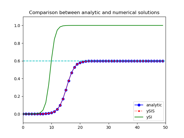
plt.title("Comparison between analytic and numerical solutions")
plt.axhline(y=fsig,ls="--",c='c')  # 添加水平直线
plt.legend(loc='best') 
plt.axis([0, 50, -0.1, 1.1])
plt.show()

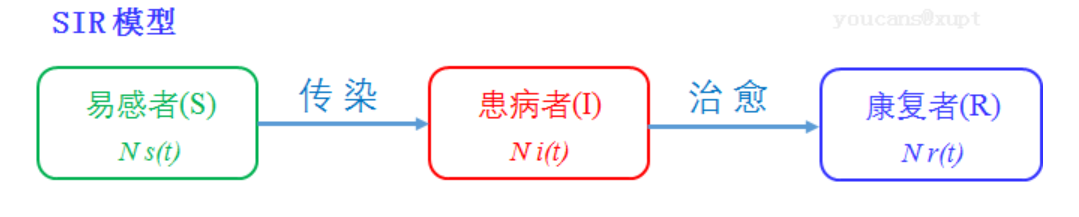
SIR模型

SIR 模型适用于具有易感者、患病者和康复者三类人群，可以治愈，且治愈后终身免疫不再复发的疾病，例如天花、肝炎、麻疹等免疫力很强的传染病。

$\left\{\begin{array}{l} \mathrm{N} \frac{\mathrm{ds}}{\mathrm{dt}}=-\mathrm{N} \lambda \mathrm{si} \\ \mathrm{Ni} \frac{\mathrm{di}}{\mathrm{dt}}=\mathrm{N} \lambda \mathrm{si}-\mu \mathrm{i} \\ \mathrm{s}(\mathrm{t})+\mathrm{i}(\mathrm{t})+\mathrm{r}(\mathrm{t})=1 \end{array}\right.$

$\left\{\begin{array}{ll} \frac{\mathrm{ds}}{\mathrm{dt}}=-\lambda \mathrm{si}, \quad \mathrm{s}(0)=\mathrm{s}_{0} \\ \frac{\mathrm{di}}{\mathrm{dt}}=\lambda \mathrm{si}-\mu \mathrm{i}, & \mathrm{i}(0)=\mathrm{i}_{0} \end{array}\right.$

SIR不能求出解析解，只能通过数值计算方法求解。

# 1. SIR 模型，常微分方程组
from scipy.integrate import odeint  # 导入 scipy.integrate 模块
import numpy as np  # 导入 numpy包
import matplotlib.pyplot as plt  # 导入 matplotlib包

def dySIS(y, t, lamda, mu):  # SI/SIS 模型，导数函数
    dy_dt = lamda*y*(1-y) - mu*y  # di/dt = lamda*i*(1-i)-mu*i
    return dy_dt

def dySIR(y, t, lamda, mu):  # SIR 模型，导数函数
    i, s = y
    di_dt = lamda*s*i - mu*i  # di/dt = lamda*s*i-mu*i
    ds_dt = -lamda*s*i  # ds/dt = -lamda*s*i
    return np.array([di_dt,ds_dt])

# 设置模型参数
number = 1e5  # 总人数
lamda = 0.2  # 日接触率, 患病者每天有效接触的易感者的平均人数
sigma = 2.5  # 传染期接触数
mu = lamda/sigma  # 日治愈率, 每天被治愈的患病者人数占患病者总数的比例
fsig = 1-1/sigma
tEnd = 200  # 预测日期长度
t = np.arange(0.0,tEnd,1)  # (start,stop,step)
i0 = 1e-4  # 患病者比例的初值
s0 = 1-i0  # 易感者比例的初值
Y0 = (i0, s0)  # 微分方程组的初值

print("lamda={}\tmu={}\tsigma={}\t(1-1/sig)={}".format(lamda,mu,sigma,fsig))

# odeint 数值解，求解微分方程初值问题
ySI = odeint(dySIS, i0, t, args=(lamda,0))  # SI 模型
ySIS = odeint(dySIS, i0, t, args=(lamda,mu))  # SIS 模型
ySIR = odeint(dySIR, Y0, t, args=(lamda,mu))  # SIR 模型

# 绘图
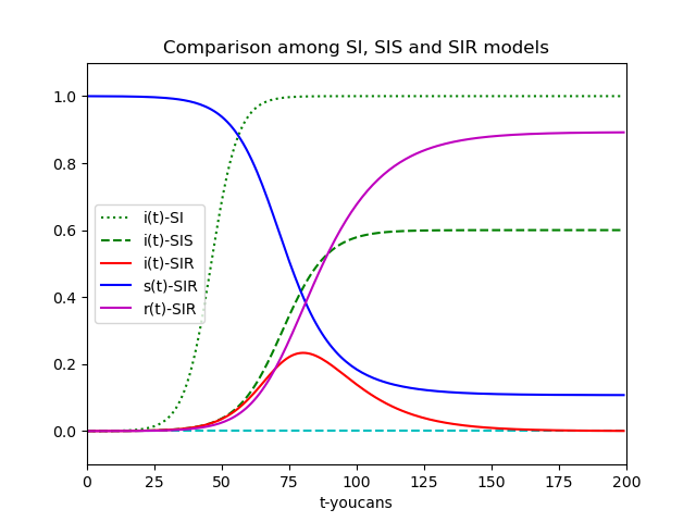
plt.title("Comparison among SI, SIS and SIR models")
plt.xlabel('t-youcans')
plt.axis([0, tEnd, -0.1, 1.1])
plt.axhline(y=0,ls="--",c='c')  # 添加水平直线
plt.plot(t, ySI, ':g', label='i(t)-SI')
plt.plot(t, ySIS, '--g', label='i(t)-SIS')
plt.plot(t, ySIR[:,0], '-r', label='i(t)-SIR')
plt.plot(t, ySIR[:,1], '-b', label='s(t)-SIR')
plt.plot(t, 1-ySIR[:,0]-ySIR[:,1], '-m', label='r(t)-SIR')
plt.legend(loc='best') 
plt.show()

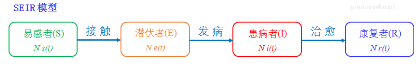
SEIR模型

SEIR 模型考虑存在易感者（Susceptible）、暴露者（Exposed）、患病者（Infectious）和康复者（Recovered）四类人群，适用于具有潜伏期、治愈后获得终身免疫的传染病。易感者（S 类）被感染后成为潜伏者（E类），随后发病成为患病者（I 类），治愈后成为康复者（R类）。这种情况更为复杂，也更为接近实际情况。

$\left\{\begin{array}{l} \mathrm{N} \frac{\mathrm{ds}}{\mathrm{dt}}=-\mathrm{N} \lambda \mathrm{si} \\ \mathrm{N} \frac{\mathrm{de}}{\mathrm{dt}}=\mathrm{N} \lambda \mathrm{si}-\mathrm{N} \delta \mathrm{e} \\ \mathrm{N} \frac{\mathrm{di}}{\mathrm{dt}}=\mathrm{N} \delta \mathrm{e}-\mathrm{N} \mu \mathrm{i} \\ \mathrm{N} \frac{\mathrm{dr}}{\mathrm{dt}}=\mathrm{N} \mu \mathrm{i} \end{array}\right.$

$\left\{\begin{array}{ll} \frac{\mathrm{ds}}{\mathrm{dt}}=-\lambda \mathrm{si}, & \mathrm{s}(0)=\mathrm{s}_{0} \\ \frac{\mathrm{de}}{\mathrm{dt}}=\lambda \mathrm{si}-\delta \mathrm{e}, & \mathrm{e}(0)=\mathrm{e}_{0} \\ \frac{\mathrm{di}}{\mathrm{dt}}=\delta \mathrm{e}-\mu \mathrm{i}, & \mathrm{i}(0)=\mathrm{i}_{0} \end{array}\right.$

# 1. SEIR 模型，常微分方程组
from scipy.integrate import odeint  # 导入 scipy.integrate 模块
import numpy as np  # 导入 numpy包
import matplotlib.pyplot as plt  # 导入 matplotlib包

def dySIS(y, t, lamda, mu):  # SI/SIS 模型，导数函数
    dy_dt = lamda*y*(1-y) - mu*y  # di/dt = lamda*i*(1-i)-mu*i
    return dy_dt

def dySIR(y, t, lamda, mu):  # SIR 模型，导数函数
    s, i = y  # youcans
    ds_dt = -lamda*s*i  # ds/dt = -lamda*s*i
    di_dt = lamda*s*i - mu*i  # di/dt = lamda*s*i-mu*i
    return np.array([ds_dt,di_dt])

def dySEIR(y, t, lamda, delta, mu):  # SEIR 模型，导数函数
    s, e, i = y  # youcans
    ds_dt = -lamda*s*i  # ds/dt = -lamda*s*i
    de_dt = lamda*s*i - delta*e  # de/dt = lamda*s*i - delta*e
    di_dt = delta*e - mu*i  # di/dt = delta*e - mu*i
    return np.array([ds_dt,de_dt,di_dt])

# 设置模型参数
number = 1e5  # 总人数
lamda = 0.3  # 日接触率, 患病者每天有效接触的易感者的平均人数
delta = 0.03  # 日发病率，每天发病成为患病者的潜伏者占潜伏者总数的比例
mu = 0.06  # 日治愈率, 每天治愈的患病者人数占患病者总数的比例
sigma = lamda / mu  # 传染期接触数
fsig = 1-1/sigma
tEnd = 300  # 预测日期长度
t = np.arange(0.0,tEnd,1)  # (start,stop,step)
i0 = 1e-3  # 患病者比例的初值
e0 = 1e-3  # 潜伏者比例的初值
s0 = 1-i0  # 易感者比例的初值
Y0 = (s0, e0, i0)  # 微分方程组的初值

# odeint 数值解，求解微分方程初值问题
ySI = odeint(dySIS, i0, t, args=(lamda,0))  # SI 模型
ySIS = odeint(dySIS, i0, t, args=(lamda,mu))  # SIS 模型
ySIR = odeint(dySIR, (s0,i0), t, args=(lamda,mu))  # SIR 模型
ySEIR = odeint(dySEIR, Y0, t, args=(lamda,delta,mu))  # SEIR 模型

# 输出绘图
print("lamda={}\tmu={}\tsigma={}\t(1-1/sig)={}".format(lamda,mu,sigma,fsig))
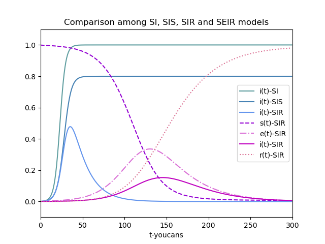
plt.title("Comparison among SI, SIS, SIR and SEIR models")
plt.xlabel('t-youcans')
plt.axis([0, tEnd, -0.1, 1.1])
plt.plot(t, ySI, 'cadetblue', label='i(t)-SI')
plt.plot(t, ySIS, 'steelblue', label='i(t)-SIS')
plt.plot(t, ySIR[:,1], 'cornflowerblue', label='i(t)-SIR')
# plt.plot(t, 1-ySIR[:,0]-ySIR[:,1], 'cornflowerblue', label='r(t)-SIR')
plt.plot(t, ySEIR[:,0], '--', color='darkviolet', label='s(t)-SIR')
plt.plot(t, ySEIR[:,1], '-.', color='orchid', label='e(t)-SIR')
plt.plot(t, ySEIR[:,2], '-', color='m', label='i(t)-SIR')
plt.plot(t, 1-ySEIR[:,0]-ySEIR[:,1]-ySEIR[:,2], ':', color='palevioletred', label='r(t)-SIR')
plt.legend(loc='right') 
plt.show()

SEIR改进模型

可见新冠疫情 SEIR 改进模型，在此不进行过多的详述。

2.4 差分方程（人口模型）

对连续系统进行离散化处理。

将人按年龄分为n组，每组该年人口总数为 $a_i$ ，普遍存活率为 $C_i$ ,普遍生育率为 $b_i$ ，下一年每组人口总数为 $a_i'$ ，

$\left\{\begin{array}{l}a_{i}^{\prime}=a_{i-1} c_{i-1}, i=2,3, \ldots, n \\ a_{1}^{\prime}=\sum_{i=1}^{n} a_{i} b_{i}\end{array}\right.$

\vec{a^{'}} = (\begin{array}{ccccc} b_{1} & b_{2} & \dots & b_{n - 1} & b_{n} \\ c_{1} & 0 & \dots & 0 & 0 \\ 0 & c_{2} & \dots & 0 & 0 \\ ⋮ & ⋮ & ⋮ \\ 0 & 0 & \dots & c_{n - 1} & 0 \end{array}) {(a_{1}, a_{2}, \dots, a_{n})}^{T}

$\overrightarrow{a^{\prime}}=\left(\begin{array}{ccccc} b_{1} & b_{2} & \ldots & b_{n-1} & b_{n} \\ c_{1} & 0 & \ldots & 0 & 0 \\ 0 & c_{2} & \ldots & 0 & 0 \\ \vdots & \vdots & & \vdots & \\ 0 & 0 & \ldots & c_{n-1} & 0 \end{array}\right)\left(a_{1}, a_{2}, \ldots, a_{n}\right)^{T}$

该式中左边的矩阵就旦Leslie矩阵.

2.5 数值方法

数值逼近方法

（1）梯度下降（寻找极值）

批量梯度下降法，随机梯度下降法，小批量梯度下降法

（2）牛顿法（寻找极值）

（3）欧拉法（定积分求解）

（4）龙格库塔法（定积分求解）

上一篇爬取 flbook 文档

下一篇批量提取pdf内的特定数据

本文作者：tlott

本文链接：https://www.cnblogs.com/tlott/p/16628092.html

posted @ 2022-08-26 16:46 tlott 阅读(201) 评论(0) 编辑收藏举报

刷新页面返回顶部

登录后才能查看或发表评论，立即登录或者逛逛博客园首页

tlott

第二章 微分方程与差分方程模型

第二章 微分方程与差分方程模型

2.1 常微分方程的求解

2.1.1 符号解求解

例1（符号解）

例2（符号解）

2.1.2 数值解求解

例1

例2

2.1.3 高阶微分方程求解

例1

2.2 偏微分方程的求解

2.2.1 例1

2.2.2 例2

2.3 微分方程案例

2.3.1 人口增长模型

Malthus Model

原理

局限性

Logisitc Model

原理

应用场景

2.3.2 放射问题

2.3.3 新冠传播模型

SI模型

SIS模型

SIR模型

SEIR模型

SEIR改进模型

2.4 差分方程（人口模型）

2.5 数值方法

数值逼近方法

公告

搜索

常用链接

随笔分类

随笔档案

阅读排行榜

评论排行榜

推荐排行榜

最新评论

第二章微分方程与差分方程模型

第二章微分方程与差分方程模型