
线性分类-感知机
对于数据集\(D={(x_1,y_1),\cdots,(x_N,y_N)}\)而言,其中\(y_i\)取值为\(({+1,-1})\)。而感知机就是寻找一个超平面,可以将上述数据集完全分开成两类。而完成输入空间到输出空间的映射函数如下
\[f(x)=sign(\mathbf{w}^T\mathbf{x}+b)
\]
感知机是一种线性分类模型,从数据集中所需要得到的就是超平面\(\mathbf{w^Tx}+b=0\),其中\(\mathbf{w}\)表示该超平面的法向量,\(b\)是该超平面的截距,这个超平面将特征空间划分为两个部分。而参数\(\mathbf{w}\)和\(b\)是在下面的损失函数最小的条件下得到的。
\[loss(\mathbf{w})=\sum_{i=1}^{N}I(y_{i}\mathbf{w}^T\mathbf{x}<0)
\]
若预测为正,而\(y_i\)本来为负,那么就是错误分类的点,那么就需要不断调整错误分类的点,从而得到所需要的超平面,由此可知感知机的思想就是错误驱动。对上式进行进一步的化简可以得到损失函数
\[L(\mathbf{w})=\sum_{x_i \in M}-y_i\mathbf{w}^Tx_i
\]
其中\(M\)表示错误分类的点的集合。借助随机梯度下降法得到系数更新公式。
\[w \leftarrow w+\lambda \frac{\partial L(\mathbf{w})}{\partial\mathbf{w}}\\
b \leftarrow b + \lambda \frac{\partial{L(\mathbf{w})}}{\partial{b}}
\]
其中\(\lambda\)表示学习率.而相应的梯度值如下
\[\frac{\partial{L(\mathbf{w})}}{\partial{\mathbf{w}}}=-\sum_{x_i \in M}x_iy_i\\
\frac{\partial{L(w)}}{\partial{b}}=-\sum_{x_i \in M}y_i
\]
不断迭代更新直到没有误分类的点。因而感知机算法要求数据集是完全可分的。
相应的代码实现如下:
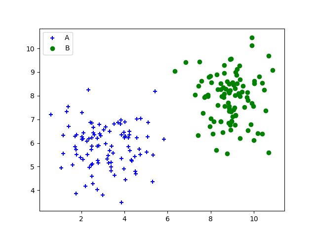
先产生数据集:
    dot_num = 100
    x_p = np.random.normal(3., 1, dot_num)
    y_p = np.random.normal(6., 1, dot_num)
    y = np.ones(dot_num)
    C1 = np.array([x_p, y_p, y]).T

    x_n = np.random.normal(9., 1, dot_num)
    y_n = np.random.normal(8., 1, dot_num)
    y = np.zeros(dot_num)-1
    C2 = np.array([x_n, y_n, y]).T

    plt.scatter(C1[:, 0], C1[:, 1], c='b', marker='+', label='A')
    plt.scatter(C2[:, 0], C2[:, 1], c='g', marker='o', label='B')
    plt.legend()
    data_set = np.concatenate((C1, C2), axis=0)
    '随机扰乱数据集'
    np.random.shuffle(data_set)
然后在训练集上训练算法
class Perception():
    def __init__(self):
        self.weight = None
        self.bias = None

    def sign(self, value):
        return 1 if value >= 0 else -1

    def train(self, data_set, labels):
        lr = 0.01
        data_set = np.array(data_set)
        n = data_set.shape[0]
        m = data_set.shape[1]
        weights = np.zeros(m)
        bias = 0
        i = 0
        while i < n:
            if (labels[i] * self.sign(np.dot(weights, data_set[i]) + bias) == -1):
                weights = weights + lr * labels[i] * data_set[i]
                bias = bias + lr * labels[i]
                i = 0
            else:
                i += 1
        self.weight = weights
        self.bias = bias

    def predict(self, data):
        if (self.weight is not None and self.bias is not None):
            return self.sign(np.dot(self.weight, data) + self.bias)
        else:
            return 0
最后得到结果如下
weights is:  [-0.3495279   0.02419943]
bias is:  1.9900000000000015
完整代码如下
import numpy as np
import matplotlib.pyplot as plt

class Perception():
    def __init__(self):
        self.weight = None
        self.bias = None

    def sign(self, value):
        return 1 if value >= 0 else -1

    def train(self, data_set, labels):
        lr = 0.01
        data_set = np.array(data_set)
        n = data_set.shape[0]
        m = data_set.shape[1]
        weights = np.zeros(m)
        bias = 0
        i = 0
        while i < n:
            if (labels[i] * self.sign(np.dot(weights, data_set[i]) + bias) == -1):
                weights = weights + lr * labels[i] * data_set[i]
                bias = bias + lr * labels[i]
                i = 0
            else:
                i += 1
        self.weight = weights
        self.bias = bias

    def predict(self, data):
        if (self.weight is not None and self.bias is not None):
            return self.sign(np.dot(self.weight, data) + self.bias)
        else:
            return 0

if __name__ == "__main__":

    dot_num = 100
    x_p = np.random.normal(3., 1, dot_num)
    y_p = np.random.normal(6., 1, dot_num)
    y = np.ones(dot_num)
    C1 = np.array([x_p, y_p, y]).T

    x_n = np.random.normal(9., 1, dot_num)
    y_n = np.random.normal(8., 1, dot_num)
    y = np.zeros(dot_num)-1
    C2 = np.array([x_n, y_n, y]).T

    plt.scatter(C1[:, 0], C1[:, 1], c='b', marker='+', label='A')
    plt.scatter(C2[:, 0], C2[:, 1], c='g', marker='o', label='B')
    plt.legend()
    data_set = np.concatenate((C1, C2), axis=0)
    '随机扰乱数据集'
    np.random.shuffle(data_set)
    perception = Perception()
    perception.train(data_set[:,0:2], data_set[:, 2])
    print("weights is: ", perception.weight)
    print("bias is: ", perception.bias)
    plt.show()

 浙公网安备 33010602011771号