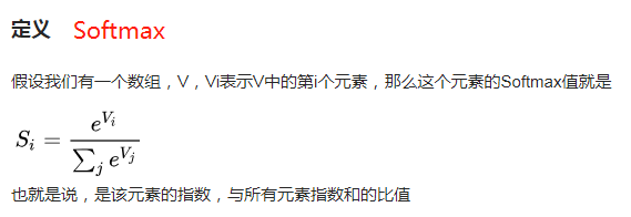
机器学习_线性回归和逻辑回归_案例实战：Python实现逻辑回归与梯度下降策略_项目实战：使用逻辑回归判断信用卡欺诈检测

线性回归：

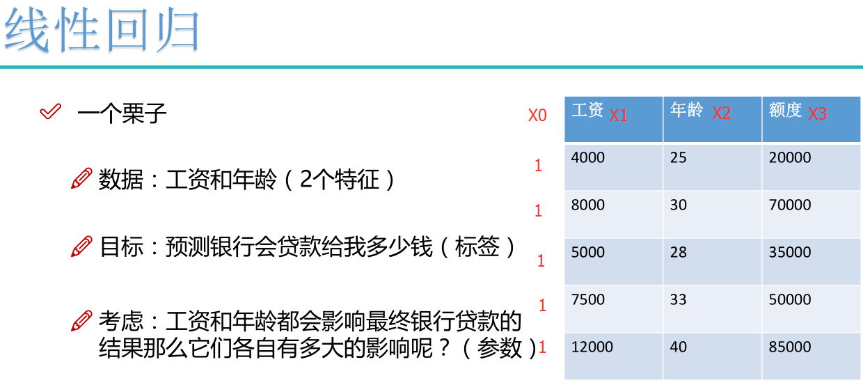
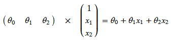
注：为偏置项，这一项的x的值假设为[1,1,1,1,1....]

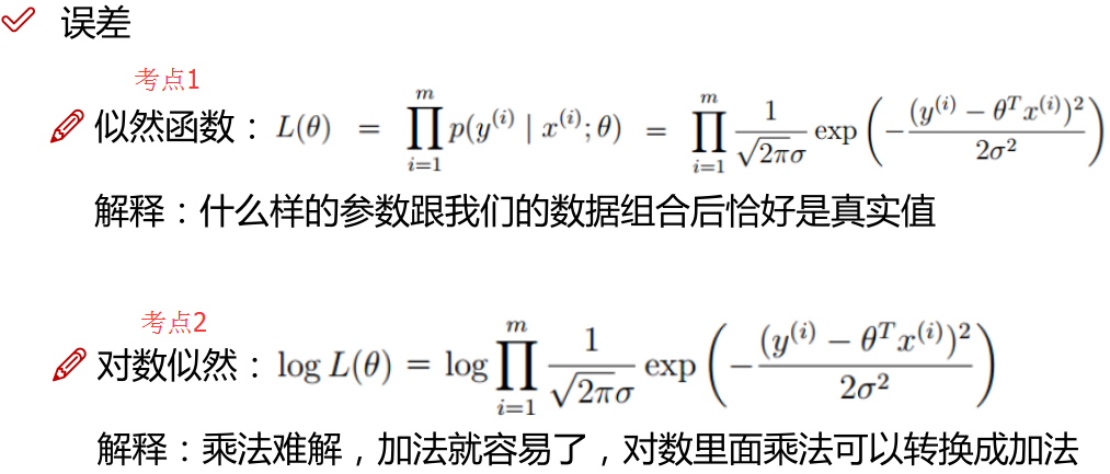
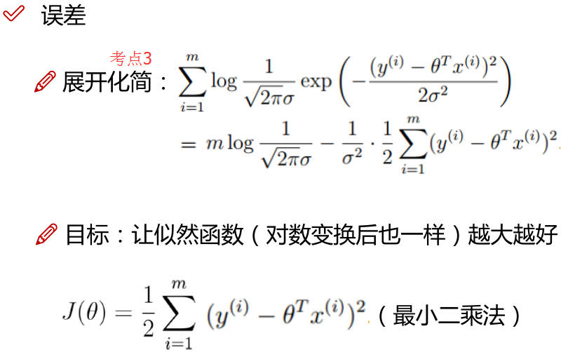
注：为使似然函数越大，则需要最小二乘法函数越小越好

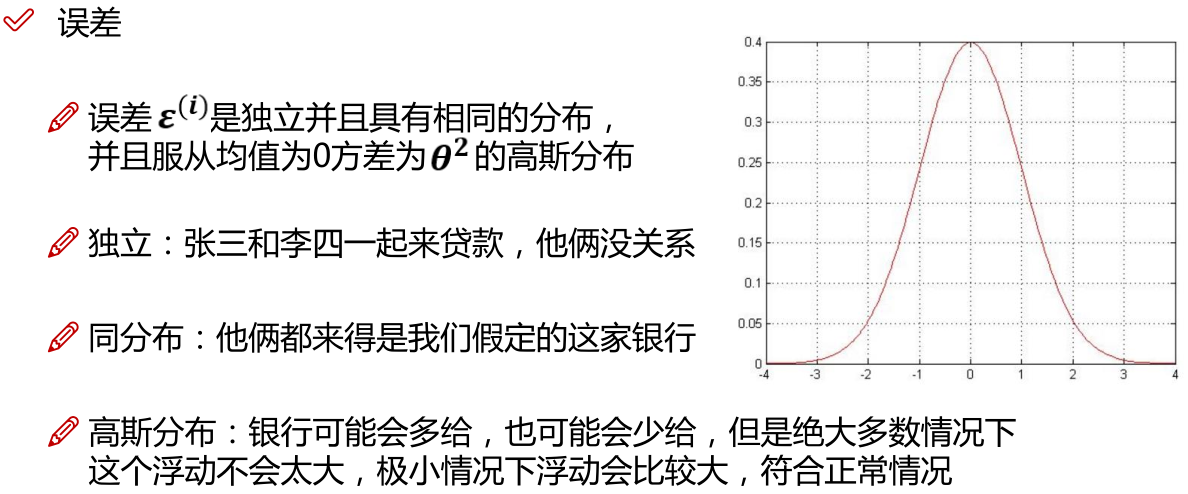
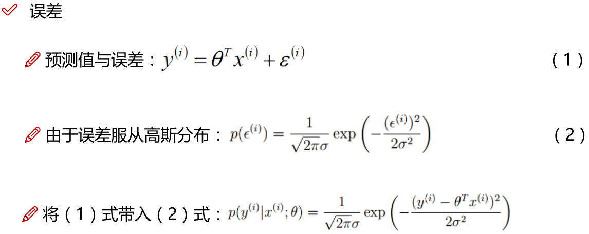
线性回归中为什么选用平方和作为误差函数？假设模型结果与测量值误差满足，均值为0的高斯分布，即正态分布。这个假设是靠谱的，符合一般客观统计规律。若使模型与测量数据最接近，那么其概率积就最大。概率积，就是概率密度函数的连续积，这样，就形成了一个最大似然函数估计。对最大似然函数估计进行推导，就得出了推导后结果：平方和最小公式

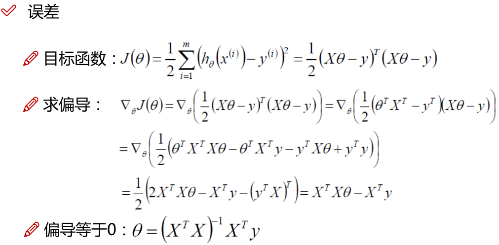
注：

1.x的平方等于x的转置乘以x。

2.机器学习中普遍认为函数属于凸函数（凸优化问题），函数图形如下，从图中可以看出函数要想取到最小值或者极小值，就需要使偏导等于0。

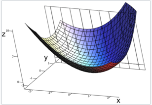
3.一些问题上没办法直接求解，则可以在上图中选一个点，依次一步步优化，取得最小值（梯度优化）

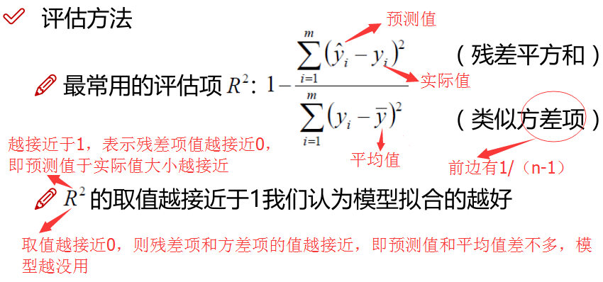
R平方是多元回归中的回归平方和占总平方和的比例，它是度量多元回归方程中拟合程度的一个统计量，反映了在因变量y的变差中被估计的回归方程所解释的比例。
R平方越接近1，表明回归平方和占总平方和的比例越大，回归线与各观测点越接近，用x的变化来解释y值变差的部分就越多，回归的拟合程度就越好。

R平方取值范围是负无穷到1，越是接近于1越好。

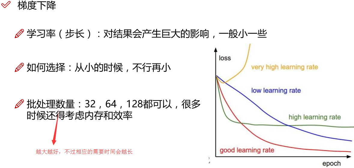
当没办法直接求解是：

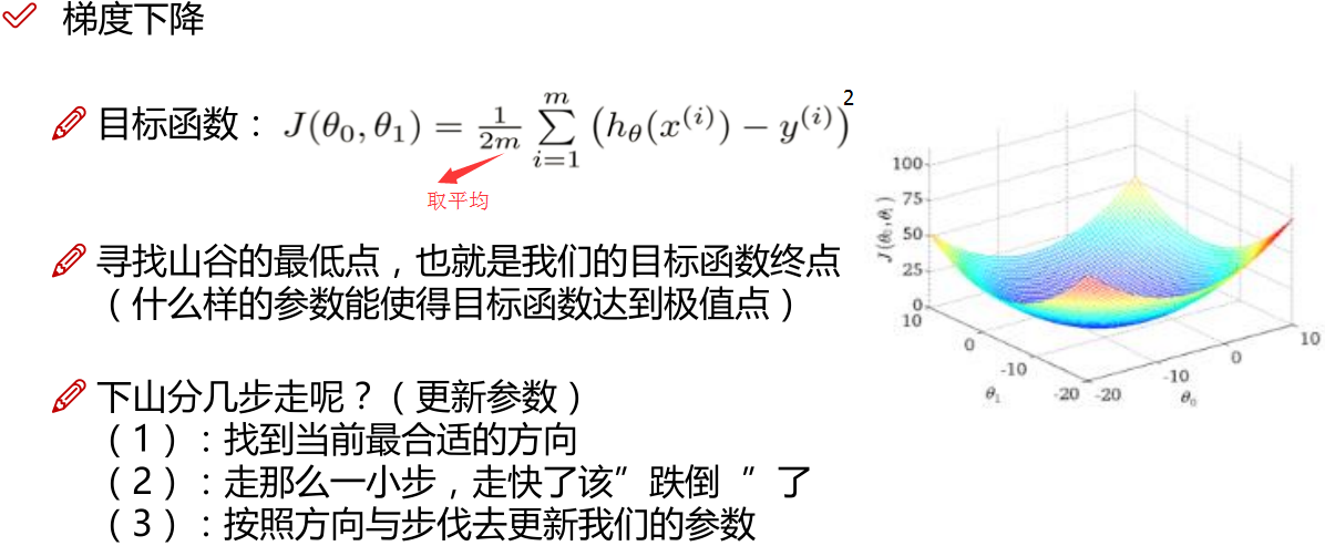
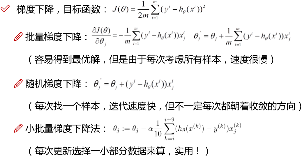
注：批量梯度下降法BGD；

　　 随机梯度下降法SGD；

　　小批量梯度下降法MBGD（在上述的批量梯度的方式中每次迭代都要使用到所有的样本，对于数据量特别大的情况，如大规模的机器学习应用，每次迭代求解所有样本需要花费大量的计算成本。是否可以在每次的迭代过程中利用部分样本代替所有的样本呢？基于这样的思想，便出现了mini-batch的概念。假设训练集中的样本的个数为1000，则每个mini-batch只是其一个子集，假设，每个mini-batch中含有10个样本，这样，整个训练数据集可以分为100个mini-batch。）

点击查看：

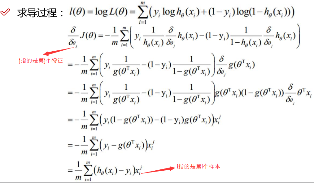
逻辑回归：

线性回归的应用场合大多是回归分析，一般不用在分类问题上，原因可以概括为以下两个：
1）回归模型是连续型模型，即预测出的值都是连续值（实数值），非离散值；
2）预测结果受样本噪声的影响比较大。

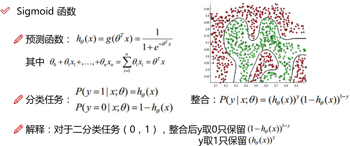
LR本质上还是线性回归，只是特征到结果的映射过程中加了一层函数映射，即sigmoid函数，即先把特征线性求和，然后使用sigmoid函数将线性和约束至(0,1)之间，结果值用于二分类。线性回归，采用的是平方损失函数。而逻辑回归采用的是对数损失函数。

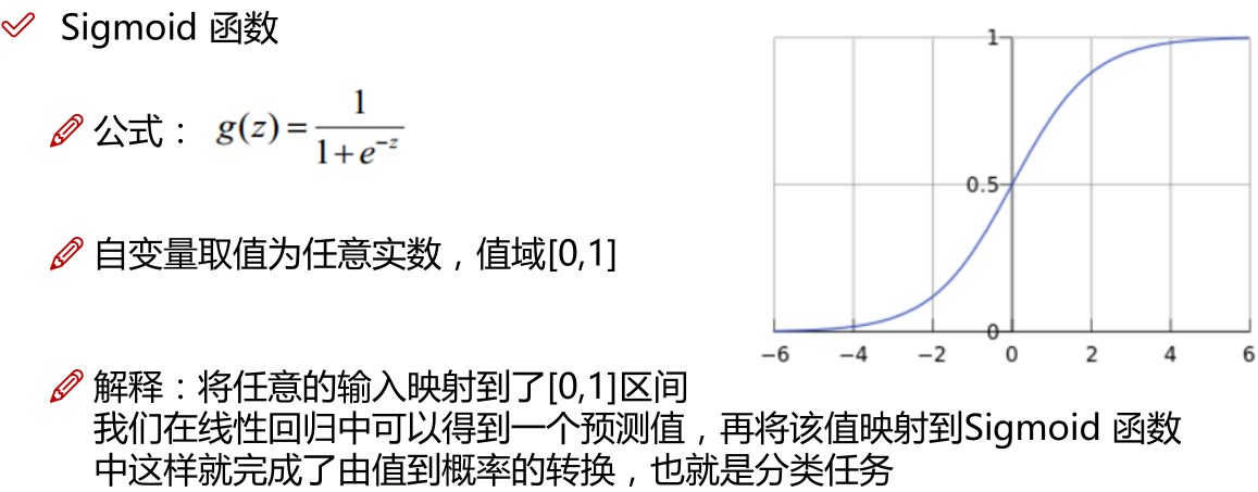
注：Z指的是线性回归的输出

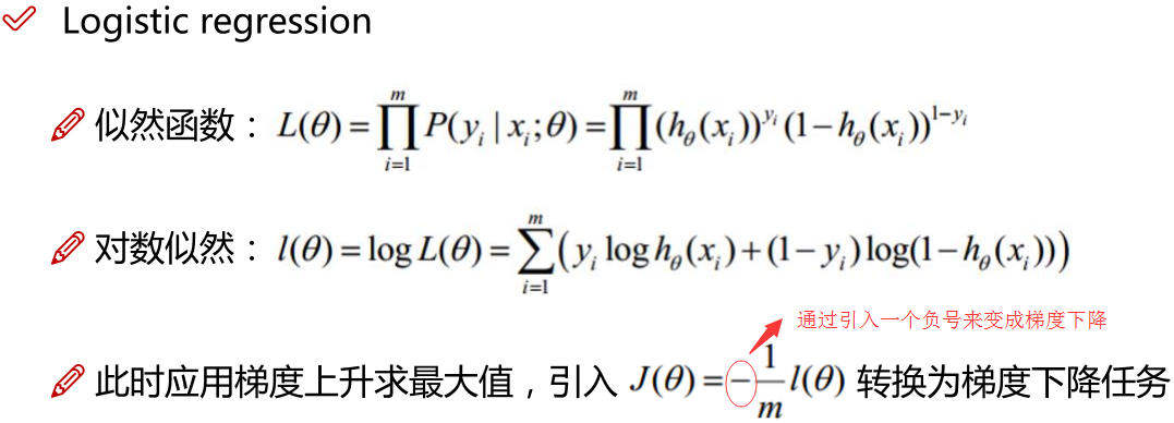
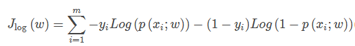
注：对数似然加负号为逻辑回归的损失函数，如下所示

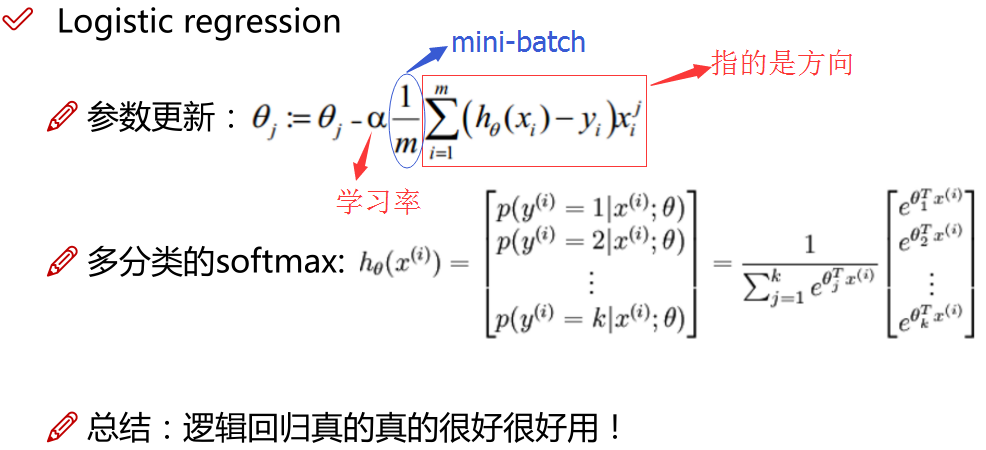
sigmoid用来解决二分类问题，softmax解决多分类问题，sigmoid是softmax的特殊情况。

核函数的物理意义？

映射到高维，使其变得线性可分。什么是高维？如一个一维数据特征x，转换为（x，x^2, x^3），就成为了一个三维特征，且线性无关。一个一维特征线性不可分的特征，在高维，就可能线性可分了。

对于非线性问题逻辑Regression问题的常规步骤为：

寻找h函数（即hypothesis）；对非线性问题的处理方式不同，LR主要靠特征构造，必须组合交叉特征，特征离散化。SVM也可以这样，还可以通过kernel
构造J函数（损失函数）；
想办法使得J函数最小并求得回归参数（θ）

LR的优缺点

优点

一、预测结果是界于0和1之间的概率；
二、可以适用于连续性和类别性自变量；
三、容易使用和解释；

缺点

1）对模型中自变量多重共线性较为敏感，例如两个高度相关自变量同时放入模型，可能导致较弱的一个自变量回归符号不符合预期，符号被扭转。需要利用因子分析或者变量聚类分析等手段来选择代表性的自变量，以减少候选变量之间的相关性；

2）预测结果呈“S”型，因此从log(odds)向概率转化的过程是非线性的，在两端随着log(odds)值的变化，概率变化很小，边际值太小，slope太小，而中间概率的变化很大，很敏感。导致很多区间的变量变化对目标概率的影响没有区分度，无法确定阀值。

为什么做回归分析和逻辑回归时要考虑消除多重共线性？

回归方程的解释，比如第一个beta1 意义是在保持其他自变量不变的情况下，X1每增加一个单位，y平均增加一个单位，记得是平均。我们进行回归分析需要了解每个自变量对因变量的单纯效应，多重共线性就是说自变量间存在某种函数关系，如果你的两个自变量间（X1和X2）存在函数关系，那么X1改变一个单位时，X2也会相应地改变，此时你无法做到固定其他条件，单独考查X1对因变量Y的作用，你所观察到的X1的效应总是混杂了X2的作用，这就造成了分析误差，使得对自变量效应的分析不准确，所以做回归分析时需要排除多重共线性的影响,就是自变量间存在很严重的相关关系。

在利用Scikit-Learn对数据进行逻辑回归之前。首先进行特征筛选。特征筛选的方法很多，主要包含在Scikit-Learn的feature-selection库中，比较简单的有通过 F 检验（f_regression）来给出各个特征的 F 值和 p 值，从而可以筛选变量（选择 F 值大的或者 p 值较小的特征）。

多重共线性的检验；

1、相关性分析，相关系数高于0.8，表明存在多重共线性；但相关系数低，并不能表示不存在多重共线性；

2、容忍度（tolerance）与方差扩大因子（VIF）。某个自变量的容忍度等于1减去该自变量为因变量而其他自变量为预测变量时所得到的线性回归模型的判定系数。容忍度越小，多重共线性越严重。通常认为容忍度小于0.1时，存在严重的多重共线性。方差扩大因子等于容忍度的倒数。显然，VIF越大，多重共线性越严重。一般认为VIF大于10时，存在严重的多重共线性。

3、回归系数的正负号与预期的相反。

多重共线性的处理方法：

（一）删除不重要的自变量
自变量之间存在共线性，说明自变量所提供的信息是重叠的，可以删除不重要的自变量减少重复信息。但从模型中删去自变量时应该注意：从实际经济分析确定为相对不重要并从偏相关系数检验证实为共线性原因的那些变量中删除。如果删除不当，会产生模型设定误差，造成参数估计严重有偏的后果。

（二）追加样本信息（不过实际操作中，这个方法实现率不高）
多重共线性问题的实质是样本信息的不充分而导致模型参数的不能精确估计，因此追加样本信息是解决该问题的一条有效途径。但是，由于资料收集及调查的困难，要追加样本信息在实践中有时并不容易。

（三）利用非样本先验信息
非样本先验信息主要来自经济理论分析和经验认识。充分利用这些先验的信息，往往有助于解决多重共线性问题。

（四）改变解释变量的形式
改变解释变量的形式是解决多重共线性的一种简易方法，例如对于横截面数据采用相对数变量，对于时间序列数据采用增量型变量。

（五）逐步回归法（此法最常用的，也最有效）
逐步回归（Stepwise Regression）是一种常用的消除多重共线性、选取“最优”回归方程的方法。其做法是将逐个引入自变量，引入的条件是该自变量经F检验是显著的，每引入一个自变量后，对已选入的变量进行逐个检验，如果原来引入的变量由于后面变量的引入而变得不再显著，那么就将其剔除。引入一个变量或从回归方程中剔除一个变量，为逐步回归的一步，每一步都要进行F 检验，以确保每次引入新变量之前回归方程中只包含显著的变量。这个过程反复进行，直到既没有不显著的自变量选入回归方程，也没有显著自变量从回归方程中剔除为止。

（六）可以做主成分回归
主成分分析法作为多元统计分析的一种常用方法在处理多变量问题时具有其一定的优越性，其降维的优势是明显的，主成分回归方法对于一般的多重共线性问题还是适用的，尤其是对共线性较强的变量之间。当采取主成分提取了新的变量后，往往这些变量间的组内差异小而组间差异大，起到了消除共线性的问题。

逻辑回归和线性回归的联系、异同？经验风险、期望风险、经验损失、结构风险之间的区别与联系？

案例实战：Python实现逻辑回归与梯度下降策略

The data

我们将建立一个逻辑回归模型来预测一个学生是否被大学录取。假设你是一个大学系的管理员，你想根据两次考试的结果来决定每个申请人的录取机会。你有以前的申请人的历史数据，你可以用它作为逻辑回归的训练集。对于每一个培训例子，你有两个考试的申请人的分数和录取决定。为了做到这一点，我们将建立一个分类模型，根据考试成绩估计入学概率。

#三大件
import numpy as np
import pandas as pd
import matplotlib.pyplot as plt
%matplotlib inline

data文件夹下 LogiReg_data.txt内容：

34.62365962451697,78.0246928153624,0
30.28671076822607,43.89499752400101,0
35.84740876993872,72.90219802708364,0
60.18259938620976,86.30855209546826,1
79.0327360507101,75.3443764369103,1
45.08327747668339,56.3163717815305,0
61.10666453684766,96.51142588489624,1
75.02474556738889,46.55401354116538,1
76.09878670226257,87.42056971926803,1
84.43281996120035,43.53339331072109,1
95.86155507093572,38.22527805795094,0
75.01365838958247,30.60326323428011,0
82.30705337399482,76.48196330235604,1
69.36458875970939,97.71869196188608,1
39.53833914367223,76.03681085115882,0
53.9710521485623,89.20735013750205,1
69.07014406283025,52.74046973016765,1
67.94685547711617,46.67857410673128,0
70.66150955499435,92.92713789364831,1
76.97878372747498,47.57596364975532,1
67.37202754570876,42.83843832029179,0
89.67677575072079,65.79936592745237,1
50.534788289883,48.85581152764205,0
34.21206097786789,44.20952859866288,0
77.9240914545704,68.9723599933059,1
62.27101367004632,69.95445795447587,1
80.1901807509566,44.82162893218353,1
93.114388797442,38.80067033713209,0
61.83020602312595,50.25610789244621,0
38.78580379679423,64.99568095539578,0
61.379289447425,72.80788731317097,1
85.40451939411645,57.05198397627122,1
52.10797973193984,63.12762376881715,0
52.04540476831827,69.43286012045222,1
40.23689373545111,71.16774802184875,0
54.63510555424817,52.21388588061123,0
33.91550010906887,98.86943574220611,0
64.17698887494485,80.90806058670817,1
74.78925295941542,41.57341522824434,0
34.1836400264419,75.2377203360134,0
83.90239366249155,56.30804621605327,1
51.54772026906181,46.85629026349976,0
94.44336776917852,65.56892160559052,1
82.36875375713919,40.61825515970618,0
51.04775177128865,45.82270145776001,0
62.22267576120188,52.06099194836679,0
77.19303492601364,70.45820000180959,1
97.77159928000232,86.7278223300282,1
62.07306379667647,96.76882412413983,1
91.56497449807442,88.69629254546599,1
79.94481794066932,74.16311935043758,1
99.2725269292572,60.99903099844988,1
90.54671411399852,43.39060180650027,1
34.52451385320009,60.39634245837173,0
50.2864961189907,49.80453881323059,0
49.58667721632031,59.80895099453265,0
97.64563396007767,68.86157272420604,1
32.57720016809309,95.59854761387875,0
74.24869136721598,69.82457122657193,1
71.79646205863379,78.45356224515052,1
75.3956114656803,85.75993667331619,1
35.28611281526193,47.02051394723416,0
56.25381749711624,39.26147251058019,0
30.05882244669796,49.59297386723685,0
44.66826172480893,66.45008614558913,0
66.56089447242954,41.09209807936973,0
40.45755098375164,97.53518548909936,1
49.07256321908844,51.88321182073966,0
80.27957401466998,92.11606081344084,1
66.74671856944039,60.99139402740988,1
32.72283304060323,43.30717306430063,0
64.0393204150601,78.03168802018232,1
72.34649422579923,96.22759296761404,1
60.45788573918959,73.09499809758037,1
58.84095621726802,75.85844831279042,1
99.82785779692128,72.36925193383885,1
47.26426910848174,88.47586499559782,1
50.45815980285988,75.80985952982456,1
60.45555629271532,42.50840943572217,0
82.22666157785568,42.71987853716458,0
88.9138964166533,69.80378889835472,1
94.83450672430196,45.69430680250754,1
67.31925746917527,66.58935317747915,1
57.23870631569862,59.51428198012956,1
80.36675600171273,90.96014789746954,1
68.46852178591112,85.59430710452014,1
42.0754545384731,78.84478600148043,0
75.47770200533905,90.42453899753964,1
78.63542434898018,96.64742716885644,1
52.34800398794107,60.76950525602592,0
94.09433112516793,77.15910509073893,1
90.44855097096364,87.50879176484702,1
55.48216114069585,35.57070347228866,0
74.49269241843041,84.84513684930135,1
89.84580670720979,45.35828361091658,1
83.48916274498238,48.38028579728175,1
42.2617008099817,87.10385094025457,1
99.31500880510394,68.77540947206617,1
55.34001756003703,64.9319380069486,1
74.77589300092767,89.52981289513276,1

View Code

import os
path = 'data' + os.sep + 'LogiReg_data.txt'
print(path)#打印出路径  data\LogiReg_data.txt
pdData = pd.read_csv(path, header=None, names=['Exam 1', 'Exam 2', 'Admitted'])#header=None不从数据中读取列名，自己指定
pdData.head()

结果：

	Exam 1	Exam 2	Admitted
0	34.623660	78.024693	0
1	30.286711	43.894998	0
2	35.847409	72.902198	0
3	60.182599	86.308552	1
4	79.032736	75.344376	1

pdData.shape#查看数据维度   (100, 3)

positive = pdData[pdData['Admitted'] == 1] # returns the subset of rows such Admitted = 1, i.e. the set of *positive* examples
negative = pdData[pdData['Admitted'] == 0] # returns the subset of rows such Admitted = 0, i.e. the set of *negative* examples
print(positive.head())
print(negative.head())
fig, ax = plt.subplots(figsize=(10,5))#设置图的大小
ax.scatter(positive['Exam 1'], positive['Exam 2'], s=30, c='b', marker='o', label='Admitted')#c指得是颜色，s指的是点大小
ax.scatter(negative['Exam 1'], negative['Exam 2'], s=30, c='r', marker='x', label='Not Admitted')
ax.legend()
ax.set_xlabel('Exam 1 Score')
ax.set_ylabel('Exam 2 Score')

结果：

      Exam 1     Exam 2  Admitted
3  60.182599  86.308552         1
4  79.032736  75.344376         1
6  61.106665  96.511426         1
7  75.024746  46.554014         1
8  76.098787  87.420570         1
       Exam 1     Exam 2  Admitted
0   34.623660  78.024693         0
1   30.286711  43.894998         0
2   35.847409  72.902198         0
5   45.083277  56.316372         0
10  95.861555  38.225278         0

View Code

Text(0,0.5,'Exam 2 Score')

The logistic regression

目标：建立分类器（求解出三个参数

设定阈值，根据阈值判断录取结果

要完成的模块

sigmoid : 映射到概率的函数
model : 返回预测结果值
cost : 根据参数计算损失
gradient : 计算每个参数的梯度方向
descent : 进行参数更新
accuracy: 计算精度

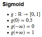
`sigmoid` 函数

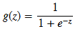
def sigmoid(z):
    return 1 / (1 + np.exp(-z))

nums = np.arange(-10, 10, step=1) #creates a vector containing 20 equally spaced values from -10 to 10
fig, ax = plt.subplots(figsize=(12,4))
ax.plot(nums, sigmoid(nums), 'r')

结果：

[<matplotlib.lines.Line2D at 0xa937a90>]

def model(X, theta):
    
    return sigmoid(np.dot(X, theta.T))

$\begin{array}{ccc} (\begin{matrix} θ_{0} & θ_{1} & θ_{2} \end{matrix}) & \times & (\begin{matrix} 1 \\ x_{1} \\ x_{2} \end{matrix}) \end{array} = θ_{0} + θ_{1} x_{1} + θ_{2} x_{2}$

pdData.insert(0, 'Ones', 1) # in a try / except structure so as not to return an error if the block si executed several times
#增加一个全1的列
print(pdData.head())
# set X (training data) and y (target variable)
orig_data = pdData.as_matrix() # convert the Pandas representation of the data to an array useful for further computations
print(orig_data)
cols = orig_data.shape[1]
print(cols)#4
X = orig_data[:,0:cols-1]
print(X)
y = orig_data[:,cols-1:cols]
print(y)
# convert to numpy arrays and initalize the parameter array theta
#X = np.matrix(X.values)
#y = np.matrix(data.iloc[:,3:4].values) #np.array(y.values)
theta = np.zeros([1, 3])
print(theta)

结果：

   Ones     Exam 1     Exam 2  Admitted
0     1  34.623660  78.024693         0
1     1  30.286711  43.894998         0
2     1  35.847409  72.902198         0
3     1  60.182599  86.308552         1
4     1  79.032736  75.344376         1
[[ 1.         34.62365962 78.02469282  0.        ]
 [ 1.         30.28671077 43.89499752  0.        ]
 [ 1.         35.84740877 72.90219803  0.        ]
 [ 1.         60.18259939 86.3085521   1.        ]
 [ 1.         79.03273605 75.34437644  1.        ]
 [ 1.         45.08327748 56.31637178  0.        ]
 [ 1.         61.10666454 96.51142588  1.        ]
 [ 1.         75.02474557 46.55401354  1.        ]
 [ 1.         76.0987867  87.42056972  1.        ]
 [ 1.         84.43281996 43.53339331  1.        ]
 [ 1.         95.86155507 38.22527806  0.        ]
 [ 1.         75.01365839 30.60326323  0.        ]
 [ 1.         82.30705337 76.4819633   1.        ]
 [ 1.         69.36458876 97.71869196  1.        ]
 [ 1.         39.53833914 76.03681085  0.        ]
 [ 1.         53.97105215 89.20735014  1.        ]
 [ 1.         69.07014406 52.74046973  1.        ]
 [ 1.         67.94685548 46.67857411  0.        ]
 [ 1.         70.66150955 92.92713789  1.        ]
 [ 1.         76.97878373 47.57596365  1.        ]
 [ 1.         67.37202755 42.83843832  0.        ]
 [ 1.         89.67677575 65.79936593  1.        ]
 [ 1.         50.53478829 48.85581153  0.        ]
 [ 1.         34.21206098 44.2095286   0.        ]
 [ 1.         77.92409145 68.97235999  1.        ]
 [ 1.         62.27101367 69.95445795  1.        ]
 [ 1.         80.19018075 44.82162893  1.        ]
 [ 1.         93.1143888  38.80067034  0.        ]
 [ 1.         61.83020602 50.25610789  0.        ]
 [ 1.         38.7858038  64.99568096  0.        ]
 [ 1.         61.37928945 72.80788731  1.        ]
 [ 1.         85.40451939 57.05198398  1.        ]
 [ 1.         52.10797973 63.12762377  0.        ]
 [ 1.         52.04540477 69.43286012  1.        ]
 [ 1.         40.23689374 71.16774802  0.        ]
 [ 1.         54.63510555 52.21388588  0.        ]
 [ 1.         33.91550011 98.86943574  0.        ]
 [ 1.         64.17698887 80.90806059  1.        ]
 [ 1.         74.78925296 41.57341523  0.        ]
 [ 1.         34.18364003 75.23772034  0.        ]
 [ 1.         83.90239366 56.30804622  1.        ]
 [ 1.         51.54772027 46.85629026  0.        ]
 [ 1.         94.44336777 65.56892161  1.        ]
 [ 1.         82.36875376 40.61825516  0.        ]
 [ 1.         51.04775177 45.82270146  0.        ]
 [ 1.         62.22267576 52.06099195  0.        ]
 [ 1.         77.19303493 70.4582      1.        ]
 [ 1.         97.77159928 86.72782233  1.        ]
 [ 1.         62.0730638  96.76882412  1.        ]
 [ 1.         91.5649745  88.69629255  1.        ]
 [ 1.         79.94481794 74.16311935  1.        ]
 [ 1.         99.27252693 60.999031    1.        ]
 [ 1.         90.54671411 43.39060181  1.        ]
 [ 1.         34.52451385 60.39634246  0.        ]
 [ 1.         50.28649612 49.80453881  0.        ]
 [ 1.         49.58667722 59.80895099  0.        ]
 [ 1.         97.64563396 68.86157272  1.        ]
 [ 1.         32.57720017 95.59854761  0.        ]
 [ 1.         74.24869137 69.82457123  1.        ]
 [ 1.         71.79646206 78.45356225  1.        ]
 [ 1.         75.39561147 85.75993667  1.        ]
 [ 1.         35.28611282 47.02051395  0.        ]
 [ 1.         56.2538175  39.26147251  0.        ]
 [ 1.         30.05882245 49.59297387  0.        ]
 [ 1.         44.66826172 66.45008615  0.        ]
 [ 1.         66.56089447 41.09209808  0.        ]
 [ 1.         40.45755098 97.53518549  1.        ]
 [ 1.         49.07256322 51.88321182  0.        ]
 [ 1.         80.27957401 92.11606081  1.        ]
 [ 1.         66.74671857 60.99139403  1.        ]
 [ 1.         32.72283304 43.30717306  0.        ]
 [ 1.         64.03932042 78.03168802  1.        ]
 [ 1.         72.34649423 96.22759297  1.        ]
 [ 1.         60.45788574 73.0949981   1.        ]
 [ 1.         58.84095622 75.85844831  1.        ]
 [ 1.         99.8278578  72.36925193  1.        ]
 [ 1.         47.26426911 88.475865    1.        ]
 [ 1.         50.4581598  75.80985953  1.        ]
 [ 1.         60.45555629 42.50840944  0.        ]
 [ 1.         82.22666158 42.71987854  0.        ]
 [ 1.         88.91389642 69.8037889   1.        ]
 [ 1.         94.83450672 45.6943068   1.        ]
 [ 1.         67.31925747 66.58935318  1.        ]
 [ 1.         57.23870632 59.51428198  1.        ]
 [ 1.         80.366756   90.9601479   1.        ]
 [ 1.         68.46852179 85.5943071   1.        ]
 [ 1.         42.07545454 78.844786    0.        ]
 [ 1.         75.47770201 90.424539    1.        ]
 [ 1.         78.63542435 96.64742717  1.        ]
 [ 1.         52.34800399 60.76950526  0.        ]
 [ 1.         94.09433113 77.15910509  1.        ]
 [ 1.         90.44855097 87.50879176  1.        ]
 [ 1.         55.48216114 35.57070347  0.        ]
 [ 1.         74.49269242 84.84513685  1.        ]
 [ 1.         89.84580671 45.35828361  1.        ]
 [ 1.         83.48916274 48.3802858   1.        ]
 [ 1.         42.26170081 87.10385094  1.        ]
 [ 1.         99.31500881 68.77540947  1.        ]
 [ 1.         55.34001756 64.93193801  1.        ]
 [ 1.         74.775893   89.5298129   1.        ]]
4
[[ 1.         34.62365962 78.02469282]
 [ 1.         30.28671077 43.89499752]
 [ 1.         35.84740877 72.90219803]
 [ 1.         60.18259939 86.3085521 ]
 [ 1.         79.03273605 75.34437644]
 [ 1.         45.08327748 56.31637178]
 [ 1.         61.10666454 96.51142588]
 [ 1.         75.02474557 46.55401354]
 [ 1.         76.0987867  87.42056972]
 [ 1.         84.43281996 43.53339331]
 [ 1.         95.86155507 38.22527806]
 [ 1.         75.01365839 30.60326323]
 [ 1.         82.30705337 76.4819633 ]
 [ 1.         69.36458876 97.71869196]
 [ 1.         39.53833914 76.03681085]
 [ 1.         53.97105215 89.20735014]
 [ 1.         69.07014406 52.74046973]
 [ 1.         67.94685548 46.67857411]
 [ 1.         70.66150955 92.92713789]
 [ 1.         76.97878373 47.57596365]
 [ 1.         67.37202755 42.83843832]
 [ 1.         89.67677575 65.79936593]
 [ 1.         50.53478829 48.85581153]
 [ 1.         34.21206098 44.2095286 ]
 [ 1.         77.92409145 68.97235999]
 [ 1.         62.27101367 69.95445795]
 [ 1.         80.19018075 44.82162893]
 [ 1.         93.1143888  38.80067034]
 [ 1.         61.83020602 50.25610789]
 [ 1.         38.7858038  64.99568096]
 [ 1.         61.37928945 72.80788731]
 [ 1.         85.40451939 57.05198398]
 [ 1.         52.10797973 63.12762377]
 [ 1.         52.04540477 69.43286012]
 [ 1.         40.23689374 71.16774802]
 [ 1.         54.63510555 52.21388588]
 [ 1.         33.91550011 98.86943574]
 [ 1.         64.17698887 80.90806059]
 [ 1.         74.78925296 41.57341523]
 [ 1.         34.18364003 75.23772034]
 [ 1.         83.90239366 56.30804622]
 [ 1.         51.54772027 46.85629026]
 [ 1.         94.44336777 65.56892161]
 [ 1.         82.36875376 40.61825516]
 [ 1.         51.04775177 45.82270146]
 [ 1.         62.22267576 52.06099195]
 [ 1.         77.19303493 70.4582    ]
 [ 1.         97.77159928 86.72782233]
 [ 1.         62.0730638  96.76882412]
 [ 1.         91.5649745  88.69629255]
 [ 1.         79.94481794 74.16311935]
 [ 1.         99.27252693 60.999031  ]
 [ 1.         90.54671411 43.39060181]
 [ 1.         34.52451385 60.39634246]
 [ 1.         50.28649612 49.80453881]
 [ 1.         49.58667722 59.80895099]
 [ 1.         97.64563396 68.86157272]
 [ 1.         32.57720017 95.59854761]
 [ 1.         74.24869137 69.82457123]
 [ 1.         71.79646206 78.45356225]
 [ 1.         75.39561147 85.75993667]
 [ 1.         35.28611282 47.02051395]
 [ 1.         56.2538175  39.26147251]
 [ 1.         30.05882245 49.59297387]
 [ 1.         44.66826172 66.45008615]
 [ 1.         66.56089447 41.09209808]
 [ 1.         40.45755098 97.53518549]
 [ 1.         49.07256322 51.88321182]
 [ 1.         80.27957401 92.11606081]
 [ 1.         66.74671857 60.99139403]
 [ 1.         32.72283304 43.30717306]
 [ 1.         64.03932042 78.03168802]
 [ 1.         72.34649423 96.22759297]
 [ 1.         60.45788574 73.0949981 ]
 [ 1.         58.84095622 75.85844831]
 [ 1.         99.8278578  72.36925193]
 [ 1.         47.26426911 88.475865  ]
 [ 1.         50.4581598  75.80985953]
 [ 1.         60.45555629 42.50840944]
 [ 1.         82.22666158 42.71987854]
 [ 1.         88.91389642 69.8037889 ]
 [ 1.         94.83450672 45.6943068 ]
 [ 1.         67.31925747 66.58935318]
 [ 1.         57.23870632 59.51428198]
 [ 1.         80.366756   90.9601479 ]
 [ 1.         68.46852179 85.5943071 ]
 [ 1.         42.07545454 78.844786  ]
 [ 1.         75.47770201 90.424539  ]
 [ 1.         78.63542435 96.64742717]
 [ 1.         52.34800399 60.76950526]
 [ 1.         94.09433113 77.15910509]
 [ 1.         90.44855097 87.50879176]
 [ 1.         55.48216114 35.57070347]
 [ 1.         74.49269242 84.84513685]
 [ 1.         89.84580671 45.35828361]
 [ 1.         83.48916274 48.3802858 ]
 [ 1.         42.26170081 87.10385094]
 [ 1.         99.31500881 68.77540947]
 [ 1.         55.34001756 64.93193801]
 [ 1.         74.775893   89.5298129 ]]
[[0.]
 [0.]
 [0.]
 [1.]
 [1.]
 [0.]
 [1.]
 [1.]
 [1.]
 [1.]
 [0.]
 [0.]
 [1.]
 [1.]
 [0.]
 [1.]
 [1.]
 [0.]
 [1.]
 [1.]
 [0.]
 [1.]
 [0.]
 [0.]
 [1.]
 [1.]
 [1.]
 [0.]
 [0.]
 [0.]
 [1.]
 [1.]
 [0.]
 [1.]
 [0.]
 [0.]
 [0.]
 [1.]
 [0.]
 [0.]
 [1.]
 [0.]
 [1.]
 [0.]
 [0.]
 [0.]
 [1.]
 [1.]
 [1.]
 [1.]
 [1.]
 [1.]
 [1.]
 [0.]
 [0.]
 [0.]
 [1.]
 [0.]
 [1.]
 [1.]
 [1.]
 [0.]
 [0.]
 [0.]
 [0.]
 [0.]
 [1.]
 [0.]
 [1.]
 [1.]
 [0.]
 [1.]
 [1.]
 [1.]
 [1.]
 [1.]
 [1.]
 [1.]
 [0.]
 [0.]
 [1.]
 [1.]
 [1.]
 [1.]
 [1.]
 [1.]
 [0.]
 [1.]
 [1.]
 [0.]
 [1.]
 [1.]
 [0.]
 [1.]
 [1.]
 [1.]
 [1.]
 [1.]
 [1.]
 [1.]]
[[0. 0. 0.]]

View Code

X[:5]

结果：

array([[ 1.        , 34.62365962, 78.02469282],
       [ 1.        , 30.28671077, 43.89499752],
       [ 1.        , 35.84740877, 72.90219803],
       [ 1.        , 60.18259939, 86.3085521 ],
       [ 1.        , 79.03273605, 75.34437644]])

View Code

y[:5]

结果：

array([[0.],
       [0.],
       [0.],
       [1.],
       [1.]])

View Code

theta#array([[0., 0., 0.]])
X.shape, y.shape, theta.shape#((100, 3), (100, 1), (1, 3))

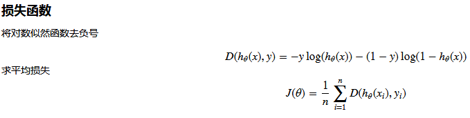注：损失函数为目标函数

def cost(X, y, theta):
    left = np.multiply(-y, np.log(model(X, theta)))
    right = np.multiply(1 - y, np.log(1 - model(X, theta)))
    return np.sum(left - right) / (len(X))

cost(X, y, theta)#0.69314718055994529

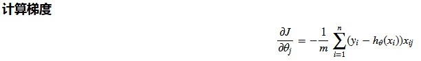
def gradient(X, y, theta):
    grad = np.zeros(theta.shape)
    error = (model(X, theta)- y).ravel()
    for j in range(len(theta.ravel())): #for each parmeter
        term = np.multiply(error, X[:,j])
        grad[0, j] = np.sum(term) / len(X)
    
    return grad

注意：.ravel用法

>>> x = np.array([[1, 2], [3, 4]])
>>> x
array([[1, 2],
       [3, 4]])
>>> x.ravel()#将多维数组降为一维，默认是行序优先
array([1, 2, 3, 4])

View Code

Gradient descent

比较3中不同梯度下降方法

STOP_ITER = 0#迭代次数标志
STOP_COST = 1#损失标志    即两次迭代目标函数之间的差异
STOP_GRAD = 2#梯度变化标志
#以上为三种停止策略，分别是按迭代次数、按损失函数的变化量、按梯度变化量
def stopCriterion(type, value, threshold):#thershold为指定阈值
    #设定三种不同的停止策略
    if type == STOP_ITER:        return value > threshold#按迭代次数停止
    elif type == STOP_COST:      return abs(value[-1]-value[-2]) < threshold#按损失函数是否改变停止
    elif type == STOP_GRAD:      return np.linalg.norm(value) < threshold#按梯度大小停止

import numpy.random
#洗牌
def shuffleData(data):
    np.random.shuffle(data)
    cols = data.shape[1]
    X = data[:, 0:cols-1]
    y = data[:, cols-1:]
    return X, y

import time

def descent(data, theta, batchSize, stopType, thresh, alpha):
    #最主要函数：梯度下降求解   batchSize：为1代表随机梯度下降，为整体值表示批量梯度下降，为某一数值表示小批量梯度下降
    #stopType：停止策略类型  thresh阈值  alpha学习率
    init_time = time.time()
    i = 0 # 迭代次数
    k = 0 # batch  迭代数据的初始量
    X, y = shuffleData(data)
    grad = np.zeros(theta.shape) # 计算的梯度
    costs = [cost(X, y, theta)] # 损失值

    
    while True:
        grad = gradient(X[k:k+batchSize], y[k:k+batchSize], theta)#batchSize为指定的梯度下降策略
        k += batchSize #取batch数量个数据
        if k >= n: 
            k = 0 
            X, y = shuffleData(data) #重新洗牌
        theta = theta - alpha*grad # 参数更新
        costs.append(cost(X, y, theta)) # 计算新的损失
        i += 1 

        if stopType == STOP_ITER:       value = i
        elif stopType == STOP_COST:     value = costs
        elif stopType == STOP_GRAD:     value = grad
        if stopCriterion(stopType, value, thresh): break
    
    return theta, i-1, costs, grad, time.time() - init_time

def runExpe(data, theta, batchSize, stopType, thresh, alpha):#损失率与迭代次数的展示函数
    #import pdb; pdb.set_trace();
    theta, iter, costs, grad, dur = descent(data, theta, batchSize, stopType, thresh, alpha)
    name = "Original" if (data[:,1]>2).sum() > 1 else "Scaled"
    name += " data - learning rate: {} - ".format(alpha)
    if batchSize==n: strDescType = "Gradient"
    elif batchSize==1:  strDescType = "Stochastic"
    else: strDescType = "Mini-batch ({})".format(batchSize)
    name += strDescType + " descent - Stop: "
    if stopType == STOP_ITER: strStop = "{} iterations".format(thresh)
    elif stopType == STOP_COST: strStop = "costs change < {}".format(thresh)
    else: strStop = "gradient norm < {}".format(thresh)
    name += strStop
    print ("***{}\nTheta: {} - Iter: {} - Last cost: {:03.2f} - Duration: {:03.2f}s".format(
        name, theta, iter, costs[-1], dur))
    fig, ax = plt.subplots(figsize=(12,4))
    ax.plot(np.arange(len(costs)), costs, 'r')
    ax.set_xlabel('Iterations')
    ax.set_ylabel('Cost')
    ax.set_title(name.upper() + ' - Error vs. Iteration')
    return theta

不同的停止策略

设定迭代次数

#选择的梯度下降方法是基于所有样本的
n=100#数据样本就100个
runExpe(orig_data, theta, n, STOP_ITER, thresh=5000, alpha=0.000001)

结果：

***Original data - learning rate: 1e-06 - Gradient descent - Stop: 5000 iterations
Theta: [[-0.00027127  0.00705232  0.00376711]] - Iter: 5000 - Last cost: 0.63 - Duration: 1.18s

array([[-0.00027127,  0.00705232,  0.00376711]])

根据损失值停止

设定阈值 1E-6, 差不多需要110 000次迭代

runExpe(orig_data, theta, n, STOP_COST, thresh=0.000001, alpha=0.001)

结果：

***Original data - learning rate: 0.001 - Gradient descent - Stop: costs change < 1e-06
Theta: [[-5.13364014  0.04771429  0.04072397]] - Iter: 109901 - Last cost: 0.38 - Duration: 24.47s

array([[-5.13364014,  0.04771429,  0.04072397]])

根据梯度变化停止

设定阈值 0.05,差不多需要40 000次迭代

runExpe(orig_data, theta, n, STOP_GRAD, thresh=0.05, alpha=0.001)

结果：

***Original data - learning rate: 0.001 - Gradient descent - Stop: gradient norm < 0.05
Theta: [[-2.37033409  0.02721692  0.01899456]] - Iter: 40045 - Last cost: 0.49 - Duration: 10.79s

array([[-2.37033409,  0.02721692,  0.01899456]])

对比不同的梯度下降方法

Stochastic descent

runExpe(orig_data, theta, 1, STOP_ITER, thresh=5000, alpha=0.001)#1指的是每次只迭代1个样本

结果：

***Original data - learning rate: 0.001 - Stochastic descent - Stop: 5000 iterations
Theta: [[-0.38504802  0.09357723 -0.01034717]] - Iter: 5000 - Last cost: 1.59 - Duration: 0.42s

array([[-0.38504802,  0.09357723, -0.01034717]])

有点爆炸。。。很不稳定,再来试试把学习率调小一些

runExpe(orig_data, theta, 1, STOP_ITER, thresh=15000, alpha=0.000002)

结果：

***Original data - learning rate: 2e-06 - Stochastic descent - Stop: 15000 iterations
Theta: [[-0.00202012  0.01009114  0.00103943]] - Iter: 15000 - Last cost: 0.63 - Duration: 1.10s

array([[-0.00202012,  0.01009114,  0.00103943]])

速度快，但稳定性差，需要很小的学习率

Mini-batch descent

runExpe(orig_data, theta, 16, STOP_ITER, thresh=15000, alpha=0.001)#16指的是每次只迭代16个样本

结果：

***Original data - learning rate: 0.001 - Mini-batch (16) descent - Stop: 15000 iterations
Theta: [[-1.0352224   0.01668297  0.0124234 ]] - Iter: 15000 - Last cost: 0.57 - Duration: 1.44s

array([[-1.0352224 ,  0.01668297,  0.0124234 ]])

浮动仍然比较大，我们来尝试下对数据进行标准化将数据按其属性(按列进行)减去其均值，然后除以其方差。最后得到的结果是，对每个属性/每列来说所有数据都聚集在0附近，方差值为1

from sklearn import preprocessing as pp

scaled_data = orig_data.copy()
scaled_data[:, 1:3] = pp.scale(orig_data[:, 1:3])

runExpe(scaled_data, theta, n, STOP_ITER, thresh=5000, alpha=0.001)

结果：

***Scaled data - learning rate: 0.001 - Gradient descent - Stop: 5000 iterations
Theta: [[ 0.3080807   0.86494967  0.77367651]] - Iter: 5000 - Last cost: 0.38 - Duration: 1.13s

array([[ 0.3080807 ,  0.86494967,  0.77367651]])

它好多了！原始数据，只能达到达到0.61，而我们得到了0.38个在这里！
所以对数据做预处理是非常重要的
记住先改数据再改模型是基本套路

runExpe(scaled_data, theta, n, STOP_GRAD, thresh=0.02, alpha=0.001)

结果：

***Scaled data - learning rate: 0.001 - Gradient descent - Stop: gradient norm < 0.02
Theta: [[ 1.071  2.63   2.411]] - Iter: 59422 - Last cost: 0.22 - Duration: 12.00s

array([[ 1.071,  2.63 ,  2.411]])

更多的迭代次数会使得损失下降的更多！

theta = runExpe(scaled_data, theta, 1, STOP_GRAD, thresh=0.002/5, alpha=0.001)

结果：

***Scaled data - learning rate: 0.001 - Stochastic descent - Stop: gradient norm < 0.0004
Theta: [[ 1.14848169  2.79268789  2.5667383 ]] - Iter: 72637 - Last cost: 0.22 - Duration: 7.05s

随机梯度下降更快，但是我们需要迭代的次数也需要更多，所以还是用batch的比较合适！！！

runExpe(scaled_data, theta, 16, STOP_GRAD, thresh=0.002*2, alpha=0.001)

结果：

***Scaled data - learning rate: 0.001 - Mini-batch (16) descent - Stop: gradient norm < 0.004
Theta: [[ 1.17096801  2.83171736  2.61095087]] - Iter: 3940 - Last cost: 0.21 - Duration: 0.50s

array([[ 1.17096801,  2.83171736,  2.61095087]])

精度

#设定阈值
def predict(X, theta):
    return [1 if x >= 0.5 else 0 for x in model(X, theta)]

scaled_X = scaled_data[:, :3]
y = scaled_data[:, 3]
predictions = predict(scaled_X, theta)
correct = [1 if ((a == 1 and b == 1) or (a == 0 and b == 0)) else 0 for (a, b) in zip(predictions, y)]
accuracy = (sum(map(int, correct)) % len(correct))
print ('accuracy = {0}%'.format(accuracy))

结果：accuracy = 89%

项目实战：使用逻辑回归判断信用卡欺诈检测

故事背景:

原始数据为个人交易记录，但是考虑数据本身的隐私性，已经对原始数据进行了类似PCA的处理，现在已经把特征数据提取好了，接下来的目的就是如何建立模型使得检测的效果达到最好，这里我们虽然不需要对数据做特征提取的操作，但是面对的挑战还是蛮大的。

import pandas as pd
import matplotlib.pyplot as plt
import numpy as np

%matplotlib inline

data = pd.read_csv("creditcard.csv")
data.head()

结果：

	Time	V1	V2	V3	V4	V5	V6	V7	V8	V9	...	V21	V22	V23	V24	V25	V26	V27	V28	Amount
0	0.0	-1.359807	-0.072781	2.536347	1.378155	-0.338321	0.462388	0.239599	0.098698	0.363787	...	-0.018307	0.277838	-0.110474	0.066928	0.128539	-0.189115	0.133558	-0.021053	149.62
1	0.0	1.191857	0.266151	0.166480	0.448154	0.060018	-0.082361	-0.078803	0.085102	-0.255425	...	-0.225775	-0.638672	0.101288	-0.339846	0.167170	0.125895	-0.008983	0.014724	2.69
2	1.0	-1.358354	-1.340163	1.773209	0.379780	-0.503198	1.800499	0.791461	0.247676	-1.514654	...	0.247998	0.771679	0.909412	-0.689281	-0.327642	-0.139097	-0.055353	-0.059752	378.66
3	1.0	-0.966272	-0.185226	1.792993	-0.863291	-0.010309	1.247203	0.237609	0.377436	-1.387024	...	-0.108300	0.005274	-0.190321	-1.175575	0.647376	-0.221929	0.062723	0.061458	123.50
4	2.0	-1.158233	0.877737	1.548718	0.403034	-0.407193	0.095921	0.592941	-0.270533	0.817739	...	-0.009431	0.798278	-0.137458	0.141267	-0.206010	0.502292	0.219422	0.215153	69.99

5 rows × 31 columns

首先我们用pandas将数据读进来并显示最开始的5行，看见木有！用pandas读取数据就是这么简单！这里的数据为了考虑用户隐私等，已经通过PCA处理过了，现在大家只需要把数据当成是处理好的特征就好啦！

接下来我们核心的目的就是去检测在数据样本中哪些是具有欺诈行为的！

count_classes = pd.value_counts(data['Class'], sort = True).sort_index()#查看该列不同属性值的个数
count_classes.plot(kind = 'bar')
plt.title("Fraud class histogram")
plt.xlabel("Class")
plt.ylabel("Frequency")

结果：<matplotlib.text.Text at 0x216366d8860>

千万不要着急去用机器学习算法建模做这个分类问题。首先我们来观察一下数据的分布情况，在数据样本中有明确的label列指定了class为0代表正常情况，class为1代表发生了欺诈行为的样本。从上图中可以看出来。。。等等，你不是说有两种情况吗，为啥图上只有class为0的样本啊？再仔细看看，纳尼。。。class为1的并不是木有，而是太少了，少到基本看不出来了，那么此时我们面对一个新的挑战，样本极度不均衡，接下来我们首先要解决这个问题，这个很常见也是很头疼的问题。这里我们提出两种解决方案也是数据分析中最常用的两种方法，下采样和过采样！先挑个软柿子捏，下采样比较简单实现，咱们就先搞定第一种方案！下采样的意思就是说，不是两类数据不均衡吗，那我让你们同样少（也就是1有多少个 0就消减成多少个），这样不就均衡了吗?

补充：

Scikit-Learn-机器学习库非常实用的机器学习算法库，这里面包含了基本你觉得你能用上所有机器学习算法啦。但还远不止如此，还有很多预处理和评估的模块等你来挖掘的！

from sklearn.preprocessing import StandardScaler
#预处理模块中的标准化
data['normAmount'] = StandardScaler().fit_transform(data['Amount'].reshape(-1, 1))#fit_transform指的是对数据做变换
data = data.drop(['Time','Amount'],axis=1)
data.head()

结果：

	V1	V2	V3	V4	V5	V6	V7	V8	V9	V10	...	V21	V22	V23	V24	V25	V26	V27	V28	normAmount
0	-1.359807	-0.072781	2.536347	1.378155	-0.338321	0.462388	0.239599	0.098698	0.363787	0.090794	...	-0.018307	0.277838	-0.110474	0.066928	0.128539	-0.189115	0.133558	-0.021053	0.244964
1	1.191857	0.266151	0.166480	0.448154	0.060018	-0.082361	-0.078803	0.085102	-0.255425	-0.166974	...	-0.225775	-0.638672	0.101288	-0.339846	0.167170	0.125895	-0.008983	0.014724	-0.342475
2	-1.358354	-1.340163	1.773209	0.379780	-0.503198	1.800499	0.791461	0.247676	-1.514654	0.207643	...	0.247998	0.771679	0.909412	-0.689281	-0.327642	-0.139097	-0.055353	-0.059752	1.160686
3	-0.966272	-0.185226	1.792993	-0.863291	-0.010309	1.247203	0.237609	0.377436	-1.387024	-0.054952	...	-0.108300	0.005274	-0.190321	-1.175575	0.647376	-0.221929	0.062723	0.061458	0.140534
4	-1.158233	0.877737	1.548718	0.403034	-0.407193	0.095921	0.592941	-0.270533	0.817739	0.753074	...	-0.009431	0.798278	-0.137458	0.141267	-0.206010	0.502292	0.219422	0.215153	-0.073403

5 rows × 30 columns

下采样：

X = data.ix[:, data.columns != 'Class']
y = data.ix[:, data.columns == 'Class']

# Number of data points in the minority class
number_records_fraud = len(data[data.Class == 1])
fraud_indices = np.array(data[data.Class == 1].index)

# Picking the indices of the normal classes
normal_indices = data[data.Class == 0].index

# Out of the indices we picked, randomly select "x" number (number_records_fraud)
random_normal_indices = np.random.choice(normal_indices, number_records_fraud, replace = False)#随机选择
random_normal_indices = np.array(random_normal_indices)

# Appending the 2 indices
under_sample_indices = np.concatenate([fraud_indices,random_normal_indices])

# Under sample dataset下采样
under_sample_data = data.iloc[under_sample_indices,:]

X_undersample = under_sample_data.ix[:, under_sample_data.columns != 'Class']
y_undersample = under_sample_data.ix[:, under_sample_data.columns == 'Class']

# Showing ratio
print("Percentage of normal transactions: ", len(under_sample_data[under_sample_data.Class == 0])/len(under_sample_data))
print("Percentage of fraud transactions: ", len(under_sample_data[under_sample_data.Class == 1])/len(under_sample_data))
print("Total number of transactions in resampled data: ", len(under_sample_data))

结果：

Percentage of normal transactions:  0.5
Percentage of fraud transactions:  0.5
Total number of transactions in resampled data:  984

很简单的实现方法，在属于0的数据中，进行随机的选择，就选跟class为1的那类样本一样多就好了，那么现在我们已经得到了两组都是非常少的数据，接下来就可以建模啦！不过在建立任何一个机器学习模型之前不要忘了一个常规的操作，就是要把数据集切分成训练集和测试集，这样会使得后续验证的结果更为靠谱。

交叉验证：

from sklearn.cross_validation import train_test_split

# Whole dataset
X_train, X_test, y_train, y_test = train_test_split(X,y,test_size = 0.3, random_state = 0)#设置随机种子，可以去掉

print("Number transactions train dataset: ", len(X_train))
print("Number transactions test dataset: ", len(X_test))
print("Total number of transactions: ", len(X_train)+len(X_test))

# Undersampled dataset
X_train_undersample, X_test_undersample, y_train_undersample, y_test_undersample = train_test_split(X_undersample
                                                                                                   ,y_undersample
                                                                                                   ,test_size = 0.3
                                                                                                   ,random_state = 0)
print("")
print("Number transactions train dataset: ", len(X_train_undersample))
print("Number transactions test dataset: ", len(X_test_undersample))
print("Total number of transactions: ", len(X_train_undersample)+len(X_test_undersample))

结果：

Number transactions train dataset:  199364
Number transactions test dataset:  85443
Total number of transactions:  284807

Number transactions train dataset:  688
Number transactions test dataset:  296
Total number of transactions:  984

建模操作：

from sklearn.linear_model import LogisticRegression#逻辑回归
from sklearn.cross_validation import KFold, cross_val_score#K折交叉验证和交叉验证评估结果两个模块

def printing_Kfold_scores(x_train_data,y_train_data):
    fold = KFold(len(y_train_data),5,shuffle=False) 

    # Different C parameters
    c_param_range = [0.01,0.1,1,10,100]#不同的惩罚力度λ，即正则化惩罚项的系数

    results_table = pd.DataFrame(index = range(len(c_param_range),2), columns = ['C_parameter','Mean recall score'])
    results_table['C_parameter'] = c_param_range

    # the k-fold will give 2 lists: train_indices = indices[0], test_indices = indices[1]
    j = 0
    for c_param in c_param_range:#用不同的正则化系数
        print('-------------------------------------------')
        print('C parameter: ', c_param)
        print('-------------------------------------------')
        print('')

        recall_accs = []
        for iteration, indices in enumerate(fold,start=1):#各个验证集循环进行交叉验证

            # Call the logistic regression model with a certain C parameter实例化逻辑回归模型
            lr = LogisticRegression(C = c_param, penalty = 'l1')#这里选择的L1惩罚，也可以选择L2

            # Use the training data to fit the model. In this case, we use the portion of the fold to train the model
            # with indices[0]. We then predict on the portion assigned as the 'test cross validation' with indices[1]
            lr.fit(x_train_data.iloc[indices[0],:],y_train_data.iloc[indices[0],:].values.ravel())

            # Predict values using the test indices in the training data
            y_pred_undersample = lr.predict(x_train_data.iloc[indices[1],:].values)

            # Calculate the recall score and append it to a list for recall scores representing the current c_parameter
            recall_acc = recall_score(y_train_data.iloc[indices[1],:].values,y_pred_undersample)
            recall_accs.append(recall_acc)
            print('Iteration ', iteration,': recall score = ', recall_acc)

        # The mean value of those recall scores is the metric we want to save and get hold of.
        results_table.ix[j,'Mean recall score'] = np.mean(recall_accs)
        j += 1
        print('')
        print('Mean recall score ', np.mean(recall_accs))
        print('')

    best_c = results_table.loc[results_table['Mean recall score'].idxmax()]['C_parameter']
    
    # Finally, we can check which C parameter is the best amongst the chosen.
    print('*********************************************************************************')
    print('Best model to choose from cross validation is with C parameter = ', best_c)
    print('*********************************************************************************')
    
    return best_c

best_c = printing_Kfold_scores(X_train_undersample,y_train_undersample)

上述代码中做了一件非常常规的事情，就是对于一个模型，咱们再选择一个算法的时候伴随着很多的参数要调节，那么如何找到最合适的参数可不是一件简单的事，依靠经验值并不是十分靠谱，通常情况下我们需要大量的实验也就是不断去尝试最终得出这些合适的参数。不同C参数对应的最终模型效果：

-------------------------------------------
C parameter:  0.01
-------------------------------------------

Iteration  1 : recall score =  0.958904109589
Iteration  2 : recall score =  0.917808219178
Iteration  3 : recall score =  1.0
Iteration  4 : recall score =  0.972972972973
Iteration  5 : recall score =  0.954545454545

Mean recall score  0.960846151257

-------------------------------------------
C parameter:  0.1
-------------------------------------------

Iteration  1 : recall score =  0.835616438356
Iteration  2 : recall score =  0.86301369863
Iteration  3 : recall score =  0.915254237288
Iteration  4 : recall score =  0.932432432432
Iteration  5 : recall score =  0.878787878788

Mean recall score  0.885020937099

-------------------------------------------
C parameter:  1
-------------------------------------------

Iteration  1 : recall score =  0.835616438356
Iteration  2 : recall score =  0.86301369863
Iteration  3 : recall score =  0.966101694915
Iteration  4 : recall score =  0.945945945946
Iteration  5 : recall score =  0.893939393939

Mean recall score  0.900923434357

-------------------------------------------
C parameter:  10
-------------------------------------------

Iteration  1 : recall score =  0.849315068493
Iteration  2 : recall score =  0.86301369863
Iteration  3 : recall score =  0.966101694915
Iteration  4 : recall score =  0.959459459459
Iteration  5 : recall score =  0.893939393939

Mean recall score  0.906365863087

-------------------------------------------
C parameter:  100
-------------------------------------------

Iteration  1 : recall score =  0.86301369863
Iteration  2 : recall score =  0.86301369863
Iteration  3 : recall score =  0.966101694915
Iteration  4 : recall score =  0.959459459459
Iteration  5 : recall score =  0.893939393939

Mean recall score  0.909105589115

*********************************************************************************
Best model to choose from cross validation is with C parameter =  0.01
*********************************************************************************

View Code

在使用机器学习算法的时候，很重要的一部就是参数的调节，在这里我们选择使用最经典的分类算法，逻辑回归！千万别把逻辑回归当成是回归算法，它就是最实用的二分类算法！这里我们需要考虑的c参数就是正则化惩罚项的力度，那么如何选择到最好的参数呢？这里我们就需要交叉验证啦，然后用不同的C参数去跑相同的数据，目的就是去看看啥样的C参数能够使得最终模型的效果最好！可以到不同的参数对最终的结果产生的影响还是蛮大的，这里最好的方法就是用验证集去寻找了！

模型评估

模型已经造出来了，那么怎么评判哪个模型好，哪个模型不好呢？我们这里需要好好想一想！一般都是用精度来衡量，也就是常说的准确率，但是我们来想一想，我们的目的是什么呢？是不是要检测出来那些异常的样本呀！换个例子来说，假如现在医院给了我们一个任务要检测出来1000个病人中，有癌症的那些人。那么假设数据集中1000个人中有990个无癌症，只有10个有癌症，我们需要把这10个人检测出来。假设我们用精度来衡量，那么即便这10个人没检测出来，也是有 990/1000 也就是99%的精度，但是这个模型却没任何价值！这点是非常重要的，因为不同的评估方法会得出不同的答案，一定要根据问题的本质，去选择最合适的评估方法。

所以用召回率，不用精度
#Recall = TP/(TP+FN) 召回率

TP和FN的解释：

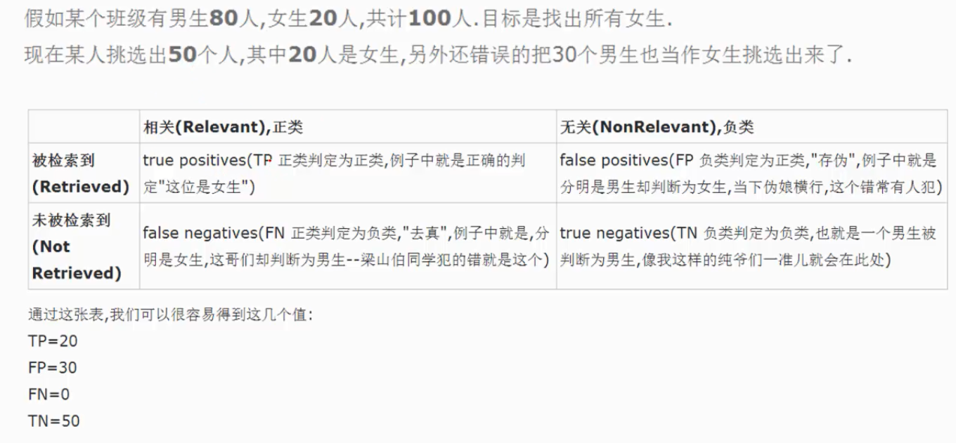
这里我们采用recall来计算模型的好坏，也就是说那些异常的样本我们的检测到了多少，这也是咱们最初的目的！这里通常用混淆矩阵来展示。

from sklearn.metrics import confusion_matrix,recall_score,classification_report #confusion_matrix指的是混淆矩阵

def plot_confusion_matrix(cm, classes,
                          title='Confusion matrix',
                          cmap=plt.cm.Blues):
    """
    This function prints and plots the confusion matrix.
    """
    plt.imshow(cm, interpolation='nearest', cmap=cmap)
    plt.title(title)
    plt.colorbar()
    tick_marks = np.arange(len(classes))
    plt.xticks(tick_marks, classes, rotation=0)
    plt.yticks(tick_marks, classes)

    thresh = cm.max() / 2.
    for i, j in itertools.product(range(cm.shape[0]), range(cm.shape[1])):
        plt.text(j, i, cm[i, j],
                 horizontalalignment="center",
                 color="white" if cm[i, j] > thresh else "black")

    plt.tight_layout()
    plt.ylabel('True label')
    plt.xlabel('Predicted label')

import itertools
lr = LogisticRegression(C = best_c, penalty = 'l1')
lr.fit(X_train_undersample,y_train_undersample.values.ravel())
y_pred_undersample = lr.predict(X_test_undersample.values)

# Compute confusion matrix
cnf_matrix = confusion_matrix(y_test_undersample,y_pred_undersample)
np.set_printoptions(precision=2)

print("Recall metric in the testing dataset: ", cnf_matrix[1,1]/(cnf_matrix[1,0]+cnf_matrix[1,1]))

# Plot non-normalized confusion matrix
class_names = [0,1]
plt.figure()
plot_confusion_matrix(cnf_matrix
                      , classes=class_names
                      , title='Confusion matrix')
plt.show()

此为下采样数据集得出的结果：

Recall metric in the testing dataset:  0.931972789116

这个图就非常漂亮了！（并不是说画的好而是展示的很直接）从图中可以清晰的看到原始数据中样本的分布以及我们的模型的预测结果。

从混淆矩阵中可以得到：

　　精度=（129+137）/（129+137+20+10）；Recall = TP/（TP+FN）=137/（137+10）=0.931972789116

利用混淆矩阵我们可以很直观的考察模型的精度以及recall，也是非常推荐大家在评估模型的时候不妨把这个图亮出来可以帮助咱们很直观的看清楚现在模型的效果以及存在的问题。

lr = LogisticRegression(C = best_c, penalty = 'l1')
lr.fit(X_train_undersample,y_train_undersample.values.ravel())
y_pred = lr.predict(X_test.values)

# Compute confusion matrix
cnf_matrix = confusion_matrix(y_test,y_pred)
np.set_printoptions(precision=2)

print("Recall metric in the testing dataset: ", cnf_matrix[1,1]/(cnf_matrix[1,0]+cnf_matrix[1,1]))

# Plot non-normalized confusion matrix
class_names = [0,1]
plt.figure()
plot_confusion_matrix(cnf_matrix
                      , classes=class_names
                      , title='Confusion matrix')
plt.show()

此为原始数据集得出的结果：Recall = TP/（TP+FN）=135/（135+12）=0.918367346939

Recall metric in the testing dataset:  0.918367346939

这可还木有完事，我们刚才只是在下采样的数据集中去进行测试的，那么这份测试还不能完全可信，因为它并不是原始的测试集，我们需要在原始的，大量的测试集中再次去衡量当前模型的效果。可以看到效果其实还不错，但是哪块有些问题呢，是不是我们误杀了很多呀，有8581个样本由0误杀成1，有些样本并不是异常的，但是并我们错误的当成了异常的，所以造成精度偏低了，这个现象其实就是下采样策略本身的一个缺陷。另外一个缺陷就是实际中工作量增加，本来只要找135个，缺误杀了8000多个，不能直接去通知8000多个客户吧，这工作量太大了，误杀已经超出了容忍范围。

补充：

上边一些列采用了下采样的方法，如果不采用下采样，直接对原始数据进行建模：

best_c = printing_Kfold_scores(X_train,y_train)

结果很差：

-------------------------------------------
C parameter:  0.01
-------------------------------------------

Iteration  1 : recall score =  0.492537313433
Iteration  2 : recall score =  0.602739726027
Iteration  3 : recall score =  0.683333333333
Iteration  4 : recall score =  0.569230769231
Iteration  5 : recall score =  0.45

Mean recall score  0.559568228405

-------------------------------------------
C parameter:  0.1
-------------------------------------------

Iteration  1 : recall score =  0.567164179104
Iteration  2 : recall score =  0.616438356164
Iteration  3 : recall score =  0.683333333333
Iteration  4 : recall score =  0.584615384615
Iteration  5 : recall score =  0.525

Mean recall score  0.595310250644

-------------------------------------------
C parameter:  1
-------------------------------------------

Iteration  1 : recall score =  0.55223880597
Iteration  2 : recall score =  0.616438356164
Iteration  3 : recall score =  0.716666666667
Iteration  4 : recall score =  0.615384615385
Iteration  5 : recall score =  0.5625

Mean recall score  0.612645688837

-------------------------------------------
C parameter:  10
-------------------------------------------

Iteration  1 : recall score =  0.55223880597
Iteration  2 : recall score =  0.616438356164
Iteration  3 : recall score =  0.733333333333
Iteration  4 : recall score =  0.615384615385
Iteration  5 : recall score =  0.575

Mean recall score  0.61847902217

-------------------------------------------
C parameter:  100
-------------------------------------------

Iteration  1 : recall score =  0.55223880597
Iteration  2 : recall score =  0.616438356164
Iteration  3 : recall score =  0.733333333333
Iteration  4 : recall score =  0.615384615385
Iteration  5 : recall score =  0.575

Mean recall score  0.61847902217

*********************************************************************************
Best model to choose from cross validation is with C parameter =  10.0
*********************************************************************************

View Code

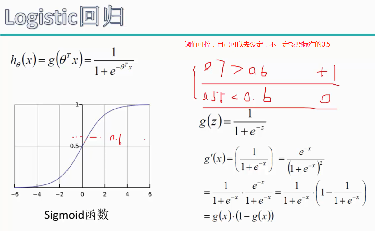
逻辑回顾阈值对结果的影响：

对于逻辑回归算法来说，我们还可以指定这样一个阈值，也就是说最终结果的概率是大于多少我们把它当成是正或者负样本。不同的阈值会对结果产生很大的影响。

lr = LogisticRegression(C = best_c, penalty = 'l1')
lr.fit(X_train,y_train.values.ravel())
y_pred_undersample = lr.predict(X_test.values)

# Compute confusion matrix
cnf_matrix = confusion_matrix(y_test,y_pred_undersample)
np.set_printoptions(precision=2)

print("Recall metric in the testing dataset: ", cnf_matrix[1,1]/(cnf_matrix[1,0]+cnf_matrix[1,1]))

# Plot non-normalized confusion matrix
class_names = [0,1]
plt.figure()
plot_confusion_matrix(cnf_matrix
                      , classes=class_names
                      , title='Confusion matrix')
plt.show()

Recall metric in the testing dataset:  0.619047619048

lr = LogisticRegression(C = 0.01, penalty = 'l1')
lr.fit(X_train_undersample,y_train_undersample.values.ravel())
y_pred_undersample_proba = lr.predict_proba(X_test_undersample.values)#由lr.predict变成lr.predict_proba

thresholds = [0.1,0.2,0.3,0.4,0.5,0.6,0.7,0.8,0.9]

plt.figure(figsize=(10,10))

j = 1
for i in thresholds:
    y_test_predictions_high_recall = y_pred_undersample_proba[:,1] > i
    
    plt.subplot(3,3,j)
    j += 1
    
    # Compute confusion matrix
    cnf_matrix = confusion_matrix(y_test_undersample,y_test_predictions_high_recall)
    np.set_printoptions(precision=2)

    print("Recall metric in the testing dataset: ", cnf_matrix[1,1]/(cnf_matrix[1,0]+cnf_matrix[1,1]))

    # Plot non-normalized confusion matrix
    class_names = [0,1]
    plot_confusion_matrix(cnf_matrix
                          , classes=class_names
                          , title='Threshold >= %s'%i)

Recall metric in the testing dataset:  1.0
Recall metric in the testing dataset:  1.0
Recall metric in the testing dataset:  1.0
Recall metric in the testing dataset:  0.986394557823
Recall metric in the testing dataset:  0.931972789116
Recall metric in the testing dataset:  0.884353741497
Recall metric in the testing dataset:  0.836734693878
Recall metric in the testing dataset:  0.748299319728
Recall metric in the testing dataset:  0.571428571429

上图中我们可以看到不用的阈值产生的影响还是蛮大的，阈值较小，意味着我们的模型非常严格宁肯错杀也不肯放过，这样会使得绝大多数样本都被当成了异常的样本，recall很高，精度稍低当阈值较大的时候我们的模型就稍微宽松些啦，这个时候会导致recall很低，精度稍高，综上当我们使用逻辑回归算法的时候，还需要根据实际的应用场景来选择一个最恰当的阈值！

过采样：

说完了下采样策略，我们继续唠一下过采样策略，跟下采样相反，现在咱们的策略是要让class为0和1的样本一样多，也就是我们需要去进行数据的生成啦!

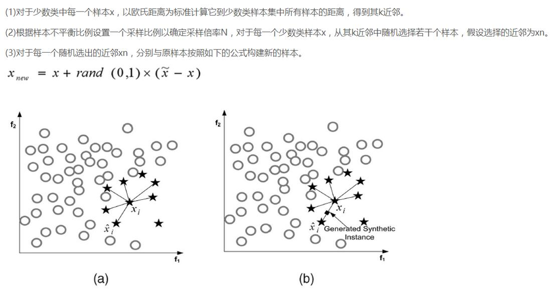
SMOTE算法是用的非常广泛的数据生成策略，流程可以参考上图，还是非常简单的，下面我们使用现成的库来帮助我们完成过采样数据生成策略。

import pandas as pd
from imblearn.over_sampling import SMOTE
from sklearn.ensemble import RandomForestClassifier
from sklearn.metrics import confusion_matrix
from sklearn.model_selection import train_test_split

credit_cards=pd.read_csv('creditcard.csv')

columns=credit_cards.columns
# The labels are in the last column ('Class'). Simply remove it to obtain features columns
features_columns=columns.delete(len(columns)-1)

features=credit_cards[features_columns]
labels=credit_cards['Class']

features_train, features_test, labels_train, labels_test = train_test_split(features, 
                                                                            labels, 
                                                                            test_size=0.2, 
                                                                            random_state=0)

oversampler=SMOTE(random_state=0)
os_features,os_labels=oversampler.fit_sample(features_train,labels_train)#只需要训练集进行过采样，测试集不要动

len(os_labels[os_labels==1])#227454

os_features = pd.DataFrame(os_features)
os_labels = pd.DataFrame(os_labels)
best_c = printing_Kfold_scores(os_features,os_labels)

结果：

-------------------------------------------
C parameter:  0.01
-------------------------------------------

Iteration  1 : recall score =  0.890322580645
Iteration  2 : recall score =  0.894736842105
Iteration  3 : recall score =  0.968861347792
Iteration  4 : recall score =  0.957595541926
Iteration  5 : recall score =  0.958430881173

Mean recall score  0.933989438728

-------------------------------------------
C parameter:  0.1
-------------------------------------------

Iteration  1 : recall score =  0.890322580645
Iteration  2 : recall score =  0.894736842105
Iteration  3 : recall score =  0.970410534469
Iteration  4 : recall score =  0.959980655302
Iteration  5 : recall score =  0.960178498807

Mean recall score  0.935125822266

-------------------------------------------
C parameter:  1
-------------------------------------------

Iteration  1 : recall score =  0.890322580645
Iteration  2 : recall score =  0.894736842105
Iteration  3 : recall score =  0.970454796946
Iteration  4 : recall score =  0.96014552489
Iteration  5 : recall score =  0.960596168431

Mean recall score  0.935251182603

-------------------------------------------
C parameter:  10
-------------------------------------------

Iteration  1 : recall score =  0.890322580645
Iteration  2 : recall score =  0.894736842105
Iteration  3 : recall score =  0.97065397809
Iteration  4 : recall score =  0.960343368396
Iteration  5 : recall score =  0.960530220596

Mean recall score  0.935317397966

-------------------------------------------
C parameter:  100
-------------------------------------------

Iteration  1 : recall score =  0.890322580645
Iteration  2 : recall score =  0.894736842105
Iteration  3 : recall score =  0.970543321899
Iteration  4 : recall score =  0.960211472725
Iteration  5 : recall score =  0.960903924995

Mean recall score  0.935343628474

*********************************************************************************
Best model to choose from cross validation is with C parameter =  100.0
*********************************************************************************

View Code

lr = LogisticRegression(C = best_c, penalty = 'l1')
lr.fit(os_features,os_labels.values.ravel())
y_pred = lr.predict(features_test.values)

# Compute confusion matrix
cnf_matrix = confusion_matrix(labels_test,y_pred)
np.set_printoptions(precision=2)

print("Recall metric in the testing dataset: ", cnf_matrix[1,1]/(cnf_matrix[1,0]+cnf_matrix[1,1]))

# Plot non-normalized confusion matrix
class_names = [0,1]
plt.figure()
plot_confusion_matrix(cnf_matrix
                      , classes=class_names
                      , title='Confusion matrix')
plt.show()

结果：

Recall metric in the testing dataset:  0.90099009901

过采样，即采用数据生成，recall召回率会相对于下采样低点，但是精度提高，误杀率降低。

我们对比一下下采样和过采样的效果，可以说recall的效果都不错，都可以检测到异常样本，但是下采样是不是误杀的比较少呀，所以如果我们可以进行数据生成，那么在处理样本数据不均衡的情况下，过采样是一个可以尝试的方案！首选也是数据生成策略，因为机器学习就是需要大量数据，数据尽量多，减少过拟合。

posted @ 2018-04-26 16:45 耐烦不急阅读(1821) 评论(0) 编辑收藏举报

会员力量，点亮园子希望

刷新页面返回顶部

机器学习_线性回归和逻辑回归_案例实战：Python实现逻辑回归与梯度下降策略_项目实战：使用逻辑回归判断信用卡欺诈检测

线性回归：

当没办法直接求解是：

点击查看：

常见的几种最优化方法（梯度下降法、牛顿法、拟牛顿法、共轭梯度法等）

梯度下降优化算法总结

逻辑回归：

LR的优缺点

优点

缺点

为什么做回归分析和逻辑回归时要考虑消除多重共线性？

多重共线性的处理方法：

案例实战：Python实现逻辑回归与梯度下降策略

The data

The logistic regression

要完成的模块

`sigmoid` 函数

Gradient descent

不同的停止策略

设定迭代次数

根据损失值停止

根据梯度变化停止

对比不同的梯度下降方法

Stochastic descent

Mini-batch descent

精度

项目实战：使用逻辑回归判断信用卡欺诈检测

故事背景:

补充：

下采样：

交叉验证：

建模操作：

模型评估

逻辑回顾阈值对结果的影响：

过采样：

公告

机器学习_线性回归和逻辑回归_案例实战：Python实现逻辑回归与梯度下降策略_项目实战：使用逻辑回归判断信用卡欺诈检测

线性回归：

当没办法直接求解是：

点击查看：

常见的几种最优化方法（梯度下降法、牛顿法、拟牛顿法、共轭梯度法等）

梯度下降优化算法总结

逻辑回归：

LR的优缺点

优点

缺点

为什么做回归分析和逻辑回归时要考虑消除多重共线性？

多重共线性的处理方法：

案例实战：Python实现逻辑回归与梯度下降策略

The data

The logistic regression

要完成的模块

sigmoid 函数

Gradient descent

不同的停止策略

设定迭代次数

根据损失值停止

根据梯度变化停止

对比不同的梯度下降方法

Stochastic descent

Mini-batch descent

精度

项目实战：使用逻辑回归判断信用卡欺诈检测

故事背景:

补充：

下采样：

交叉验证：

建模操作：

模型评估

逻辑回顾阈值对结果的影响：

过采样：

公告

`sigmoid` 函数