三、绘图和可视化之matplotlib
#matplotlib简单绘图之plot
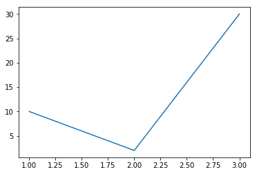
import matplotlib.pyplot as plt
a=[1,2,3]
b=[10,2,30]
plt.plot(a)#纵坐标为a的值,横坐标为a的index,即0:1,1:2,2:3
plt.show()

%matplotlib inline
#上句为jupyter中的魔法函数,不需要plt.show(),只要运行plt.plot(a,b)就会出图,在别的编译器中无法使用
plt.plot(a,b)
结果:
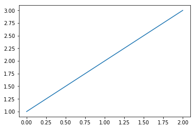
[<matplotlib.lines.Line2D at 0x8b0ae48>]
%timeit np.arange(10)
#计算出该语句的执行时间
#669 ns ± 14.7 ns per loop (mean ± std. dev. of 7 runs, 1000000 loops each)
plt.plot(a,b,'*')
结果:
[<matplotlib.lines.Line2D at 0x9d45940>]

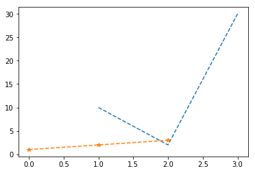
plt.plot(a,b,'--')
plt.plot(a,'*--')
结果:
[<matplotlib.lines.Line2D at 0x9e28518>]
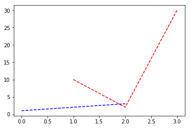
plt.plot(a,b,'r--')#改变颜色
plt.plot(a,'b--')
结果:
[<matplotlib.lines.Line2D at 0x890bcc0>]
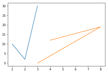
c=[4,8,3]
d=[12,19,0]
plt.plot(a,b,c,d)
结果:
[<matplotlib.lines.Line2D at 0xa368ac8>
<matplotlib.lines.Line2D at 0xa368c88>]
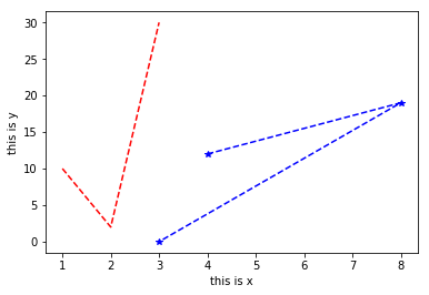
plt.plot(a,b,'r--',c,d,'b--*')
plt.xlabel('this is x')
plt.ylabel('this is y')
结果:
Text(0,0.5,'this is y')
import matplotlib.pyplot as plt
import numpy as np
x=np.linspace(0,2*np.pi,100)
print(x.size)#查看x的长度
y=np.sin(x)
print(np.pi)
plt.plot(x,y,'--')
plt.xlabel('this is x')
plt.ylabel('this is y')
plt.title('this is demo')#标题
plt.show()
结果:
100 3.141592653589793

c=[4,8,3]
d=[12,19,0]
plt.plot(a,b,label='aaaa')
plt.plot(c,d,label='bbbb')
plt.legend()#图例
结果:
<matplotlib.legend.Legend at 0x8899b38>

matplotlib简单绘图之subplot
import numpy as np
import matplotlib.pyplot as plt
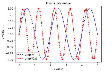
x=np.linspace(0.0,5.0)
y1=np.sin(np.pi*x)
y2=np.sin(np.pi*2*x)
#回顾plot功能
plt.plot(x,y1,'b--',label='sin(pi*x)')
plt.plot(x,y2,'r--*',label='sin(pi*2x)')
plt.ylabel('y value')
plt.xlabel('x value')
plt.title('this is x-y value')
plt.legend()
plt.show()
结果:
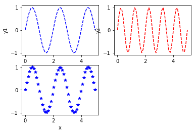
plt.subplot(2,2,1)#生成一个2行2列的subplot,这是第一个子图,位于第一行第一列
plt.plot(x,y1,'b--')
plt.ylabel('y1')
plt.subplot(222)#这是第二个子图,位于第一行第二列,plt.subplot(2,2,2),两种书写方式
plt.plot(x,y2,'r--')
plt.ylabel('y2')
plt.subplot(2,2,3)#这是第三个子图,位于第二行第一列
plt.plot(x,y1,'b*')
plt.xlabel('x')
plt.show()
结果:
figure,ax=plt.subplots()
print('ax:',ax)
print('type(ax):',type(ax))
ax.plot([1,2,3,4,5])
plt.show()
结果:
ax: AxesSubplot(0.125,0.125;0.775x0.755)
type(ax): <class 'matplotlib.axes._subplots.AxesSubplot'>

figure,ax=plt.subplots(2,2)
print('ax:',ax)
print('type(ax):',type(ax))
ax[0][0].plot(x,y1)
ax[0][1].plot(x,y2)
plt.show()
结果:
ax: [[<matplotlib.axes._subplots.AxesSubplot object at 0x0000000009D2B320>
<matplotlib.axes._subplots.AxesSubplot object at 0x0000000009E1FE10>]
[<matplotlib.axes._subplots.AxesSubplot object at 0x0000000009C621D0>

Pandas绘图之Series
import numpy as np
import pandas as pd
import matplotlib.pyplot as plt

s=pd.Series([1,2,3,4,5])
print(s.cumsum())#求每一步累加的和
结果:


0     1
1     3
2     6
3    10
4    15
dtype: int64
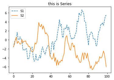
import numpy as np
import pandas as pd
import matplotlib.pyplot as plt

s1=pd.Series(np.random.randn(100)).cumsum()
s2=pd.Series(np.random.randn(100)).cumsum()
s1.plot(kind='line',grid=True,label='S1',title='this is Series',style='--')#line表示折线图(线性图),grid代表网格
s2.plot(label='S2')
plt.legend()
plt.show()
结果:
fig,ax=plt.subplots(2,1)
print(ax)
ax[0].plot(s1)
ax[1].plot(s2)
plt.show()
结果:
[<matplotlib.axes._subplots.AxesSubplot object at 0x000000000920EEF0>
<matplotlib.axes._subplots.AxesSubplot object at 0x00000000092762E8>]

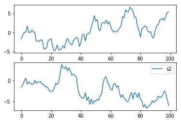
fig,ax=plt.subplots(2,1)
s1.plot(ax=ax[0],label='s1')
s2.plot(ax=ax[1],label='s2')
plt.legend()
plt.show()
结果:
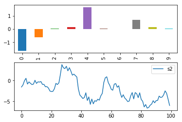
fig,ax=plt.subplots(2,1)
s1[0:10].plot(ax=ax[0],label='s1',style='*',kind='bar')
s2.plot(ax=ax[1],label='s2')
plt.legend()
plt.show()
结果:
Pandas绘图之DataFrame
import numpy as np
import pandas as pd
import matplotlib.pyplot as plt
df=pd.DataFrame(np.random.randint(1,10,40).reshape(10,4),columns=['A','B','C','D'])
print(df)
df.plot()#线形图
df.plot(kind='bar')#竖向柱形图
df.plot(kind='barh')#横向柱形图
df.plot(kind='bar',stacked=True)#堆叠形式显示的柱形图
df.plot(kind='area')#填充的线形图
plt.show()
结果:


#画出第五行
a=df.iloc[5]#取第五行
print(a)
print(type(a))#Series
df.iloc[5].plot()
# plt.plot(a)与上式相同
plt.show()
结果:

#画出每一行
for i in df.index:
    df.iloc[i].plot(label=str(i))
plt.legend()
plt.show()
结果:

# 画出第二列
print(df['B'])
df['B'].plot()
plt.show()
结果:

#画出每一列
df.plot()#默认情况下为每一列的图,省去使用for循环
plt.show()
结果:
#为了方便的画出每一行数据,省去使用for循环,可以通过转置
df.T.plot()
plt.show()
结果:
matplotlib里的直方图和密度图
直方图
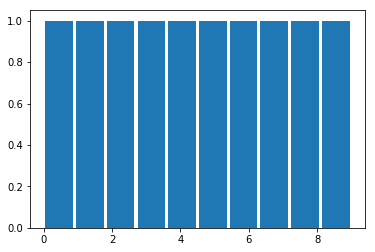
import numpy as np
import pandas as pd
import matplotlib.pyplot as plt
a=np.arange(10)
plt.hist(a,rwidth=0.9)#设置宽度为0.9
plt.show()
结果:
s=pd.Series(np.random.randn(1000))
plt.hist(s,bins=20)#分割区间设置为20
plt.show()
结果:

re=plt.hist(s,rwidth=0.9,color='r')#颜色设置为红色
print(type(re),len(re))#tuple,3
print(re[0])#代表的式频率,即指出现的次数
print(re[1])#取值间隔
print(re[2])#10个矩形
plt.show()
结果:

#线形图
s.plot()#默认为线形图
plt.show()
结果:

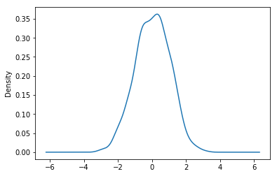
密度图
#密度图
s.plot(kind='kde')
plt.show()
结果: