A graph comprises nodes (also called vertices) connected by links (also known as edges or arcs), each node represents a random variable (or group of random variables) and the links express probabilistic relationships between these variables. The two main class of graphical models are Bayesian networks (also known as directed graphical model) and Markov random fields (also known as undirected graphical model).
Consider an arbitrary joint distribution ![]() over these variables a, b, c. By application product rule of Bayesian rule, we can write the joint distribution in the form
over these variables a, b, c. By application product rule of Bayesian rule, we can write the joint distribution in the form ![]()
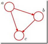
We now represent the right-hand side of the above equation in terms of a simple graphical model as the right Figure:
For each conditional distribution we add directed links (arrows) to the graph from the nodes corresponding to the variables on which the distribution is conditioned. Thus for the factor ![]() , there will be links from nodes a and b to node c. If there is a link going from a node a to a node b, then we say that node a is the parent of node b, and we say that node b is the child of node a.
, there will be links from nodes a and b to node c. If there is a link going from a node a to a node b, then we say that node a is the parent of node b, and we say that node b is the child of node a.
For the moment let us consider the joint distribution over K variables given by ![]() . By repeated application of the product rule of probability, this joint distribution can be written:
. By repeated application of the product rule of probability, this joint distribution can be written:
 We can again represent this as a directed graphical model with K nodes, with each node having an incoming links from all lower numbered nodes. We say that this graph is fully connected because there is a link between every pair of nodes. So far, we have worked with completely general joint distributions, so that the decompositions, and their representations as fully connected graphs, will be applicable to any choice of distribution.
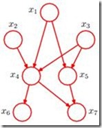
Consider the right Figure, we shall now go from graph to the corresponding representation of the joint probability distribution written in terms of the product of a set of conditional distributions, one for each node in the graph. For instance, ![]() is conditioned on
is conditioned on ![]() and
and ![]() . The joint distribution of all 7 variables is given:
. The joint distribution of all 7 variables is given:![]()
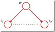
 Consider the right graphical model, the variables in the model are w and a vector of observerd data
 ![]() , when we start to deal with more complex models later in the book, we shall find it inconvenient to have to write out multiple nodes of the form
, when we start to deal with more complex models later in the book, we shall find it inconvenient to have to write out multiple nodes of the form ![]() . The distribution is given:
. The distribution is given:
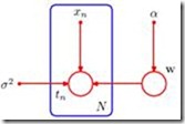
 Therefore we shall introduce a graphical notation that allows such multiple nodes to be expressed more compactly, in which we draw a single representative node
 ![]() and then surround this with a box and then surround this with a box, called a plate, labelled with N indicating that there are N nodes of this kind. In this case the graphical model becomes the right Figure.
and then surround this with a box and then surround this with a box, called a plate, labelled with N indicating that there are N nodes of this kind. In this case the graphical model becomes the right Figure.
 We shall sometimes find it helpful to make the parameters of a model, as well as its stochastic variables, explicit. In this case, the equation becomes:


