
[NLP笔记] Word Representation
Word representation is a process that transform the symbols to the machine understandable meanings. The goals of Word Representation are
- Compute word similarity
WR(Star) ≃ WR(Sun)
WR(Motel) ≃ WR(Hotel)
- Infer word relation
WR(China) − WR(Beijing) ≃ WR(Japan) - WR(Tokyo)
WR(Man) ≃ WR(King) − WR(Queen) + WR(Woman)
WR(Swimming) ≃ WR(Walking) − WR(Walk) + WR(Swim)
Now we start to discuss some ways of obtaining word representations.
1. Use a set of related words
Such as using synonyms and hypernyms to represent a word. e.g. WordNet, a resource containing synonym and hypernym sets.
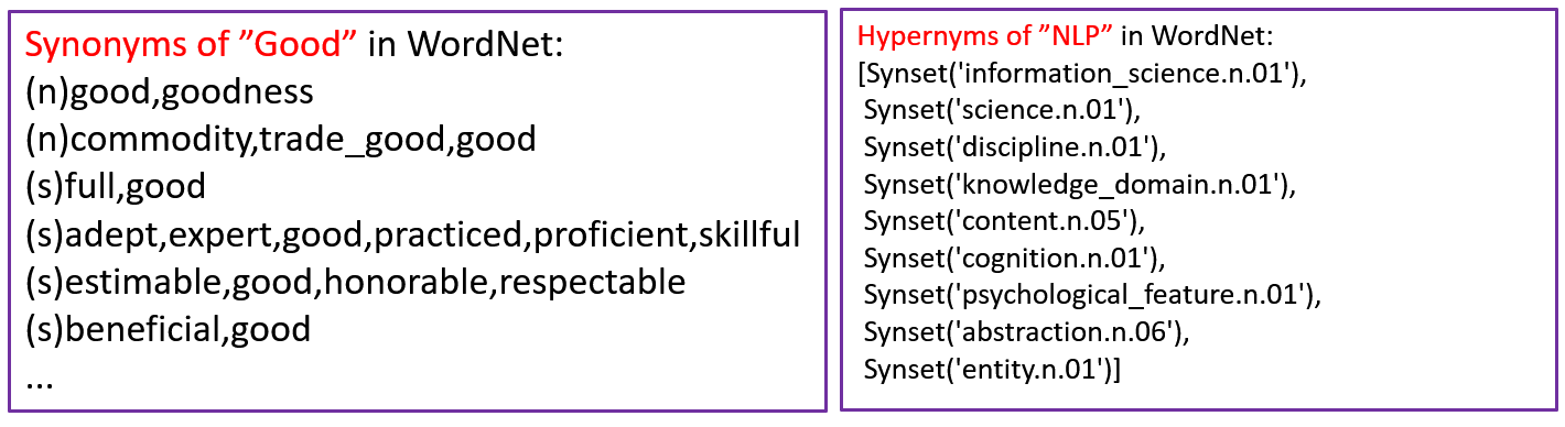
However, lots of problems exist:
-
Missing nuance
("proficient", "good") are synonyms only in some contexts
-
Missing new meanings of words
Apple (fruit → IT company)
-
Subjective
-
Data sparsity
-
Requires human labor to create and adapt
2. One-Hot Representation
Regard words as discrete symbols.
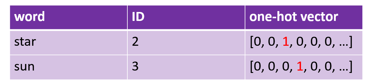
- Vector dimension = # words in vocabulary
- Token with greater ID value doesn't imply more or less important as compared with the token with less ID value.
The problem is all the vectors are orthogonal. No natural notion of similarity for one-hot vectors.
3. Represent Word by Context
Core idea is that a word's meaning is given by the words that frequently appear close-by, which is one of the most successful ideas of modern statistical NLP.
"You shall know a word by the company it keeps." (J.R. Firth 1957: 11)
2 ways to achieve this:
- Co-occurrence Counts
- Words Embeddings
Count-based distributional representation
1) Term-Term matrix
Measuring how often a word occurs with another.
where 𝐧 is the length of sentence 𝑰, 𝐦 is the length of the window.
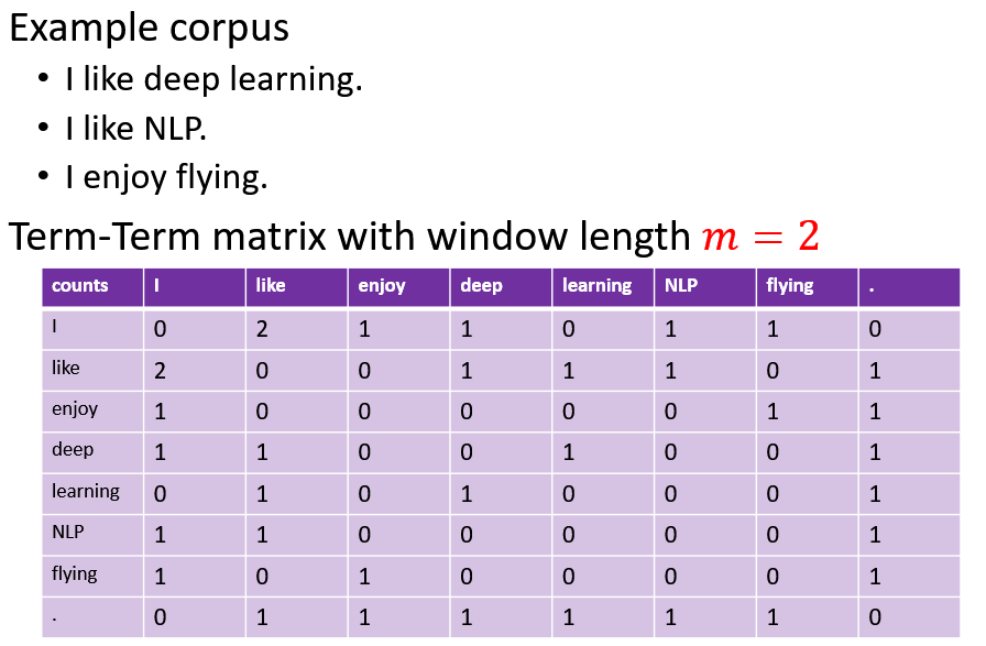
This can captures both syntactic and semantic information.
The shorter the windows, the more syntactic the representation (𝑚∈[1,3]) . The longer the windows, the more semantic the representation (𝑚∈[4,10]) .
2) Term-Document matrix
Measuring how often a word occurs in a document. Each document is a count vector in \(ℕ^𝑉\) (a column) and each word is a count vector in \(ℕ^𝐷\) (a row).

In large corpora, we expect to see that two words are similar if their vectors are similar and two documents are similar if their vectors are similar.
Given 2 word vectors 𝑣 and 𝑤, we can use the dot product to measure the similarity. We can normalize the similarity using vector's length which represents the word's frequency in documents.
Therefore, we often use cosine similarity in practice,
Problems of Count-Based Representation
- Increase in size with vocabulary
- Require a lot of storage
- sparsity issues for those less frequent words, which will causes classification models less robust
We prefer a dense vector to a sparse one, because dense vectors have a better generalization ability and short vectors are easier to use as features in machine learning.
One way to obtain dense vectors is using SVD (Singular Value Decomposition) discribed as below.
A 𝑚×𝑛 matrix \(𝑀\) can be represented as \(𝑀=𝑈Σ𝑉^∗\), where \(𝑈\) is a 𝑚×𝑘 matrix, rows corresponding to original rows, but 𝑘 columns represents a dimension in a new latent space, such that 𝑘 column vectors are orthogonal to each other.
\(Σ\) is a 𝑘×𝑘 diagonal matrix of singular values expressing the importance of each dimension.
\(𝑉^∗\) is a 𝑘×𝑛 matrix, columns corresponding to original columns, but 𝑘 rows corresponding to the singular values.
SVD can be applied to term-term matrix (co-occurrence matrix) to create dense vectors.
If 𝑘 is not small enough, we can keep the top-k singular values (like 300) to obtain a least-squares approximation to \(𝑀\). In this way, we can reduce word representation dimension.
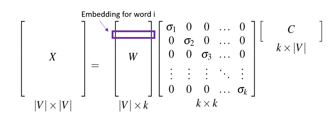
The 𝑋 in the diagram is a term-term matrix, and each row of 𝑊 is a 𝑘-dimensional representation of each word w.
However, SVD do poorly on word analogy and the matrix is high dimensional and very sparse. Besides, the computational cost is \(O(V^3)\), which is hard to accept.
Distributed Word Representation
In non-distributed or local representation, each possible value has a unique representation slot, which requires a lot of memory to process a large database than the distributed approach.
Whereas with the distributed approach, you could store all that data with just a few memory units:
Vehicle class (1= Large SUV, 0.1 = Compact, etc…), Brand, Price, Location, etc.
There are two main ways to get a distributed word representation:
- Neural Language Model
- Word Embedding
Neural Language Model
A neural language model is a language model based on neural networks, to learn distributed representations of words.
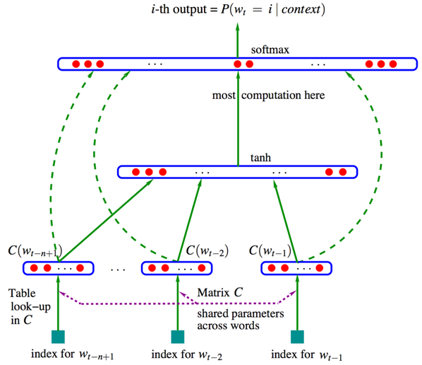
Steps:
- Associate words with distributed vectors
- Compute the joint probability of word sequences in terms of the feature vectors
- Optimize the word feature vectors (embedding matrix C) and the parameters of the loss function (the last layer, map matrix W)
But the problems is that the vocabulary size can be very large, maybe hundreds of thousands of different words. This will causes
- Too many parameters
- Lookup Table (Embedding Matrix)
- Map matrix
- Too many computation
- Non-linear operation (Tanh)
- Softmax for each words every step: Suppose there are 100,000 words in the vocabulary, we need to compute 100,000 conditional probabilities every step.
Word Embedding
Word2vec uses shallow neural networks that associate words to distributed representations. It can capture many linguistic regularities, such as "king"-"queue"="man"-"woman".
Word2vec can utilize two architectures to produce distributed representations of words:
-
Continuous bag-of-words (CBOW)
In CBOW architecture, the model predicts the target word given a window of surrounding context words according to the bag-of-word assumption: The order of context words does not influence the prediction.
\[\max P\left(w_{c} | w_{c-m}, \ldots, w_{c-1}, w_{c+1}, \ldots, w_{c+m}\right) \] -
Continuous skip-gram
In skip-gram architecture, the model predicts the context words from the target word (predict one context word each step).
\[\max P\left(w_{c-m}, \ldots, w_{c-1}, w_{c+1}, \ldots, w_{c+m} | w_{c}\right)=\prod_{-m \leq j \leq m,j\neq0} P\left(w_{c+j} | w_{c}\right) \]
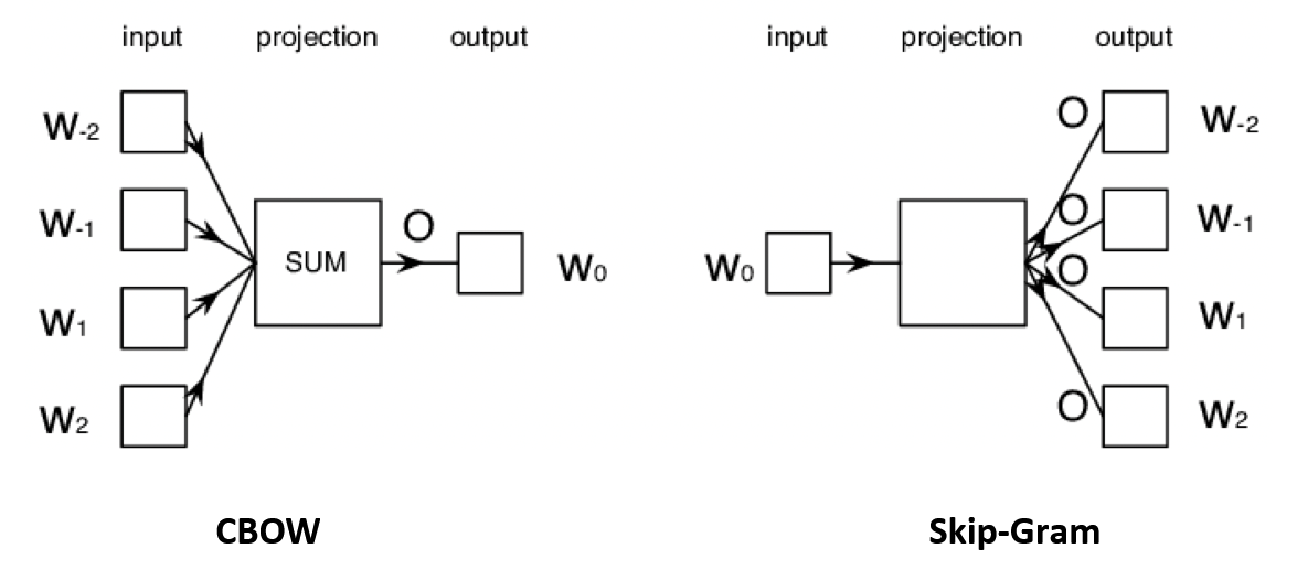
Word2vec uses a sliding window of a fixed size moving along a sentence. In each window, the middle word is the target word, other words are the context words.
Given the context words, CBOW predicts the probabilities of the target word.
While given a target word, skip-gram predicts the probabilities of the context words.
We use the softmax function to compute the prediction and use cross-entropy loss function to measure the distribution difference between the prediction and the ground truth.
Then optimize the both embedding and map matrices by optimization algorithms.
However, softmax for all the words every step depends on a huge number of model parameters when the vocabulary size is very large, which is computationally impractical.
There are two main improvement methods for word2vec:
- Negative sampling
- Hierarchical softmax
Negative sampling
The idea is, to only update a small percentage of the weights every step.
Take skip-gram for example, negative sampling aims to differentiate noisy words from the context words given the target word.
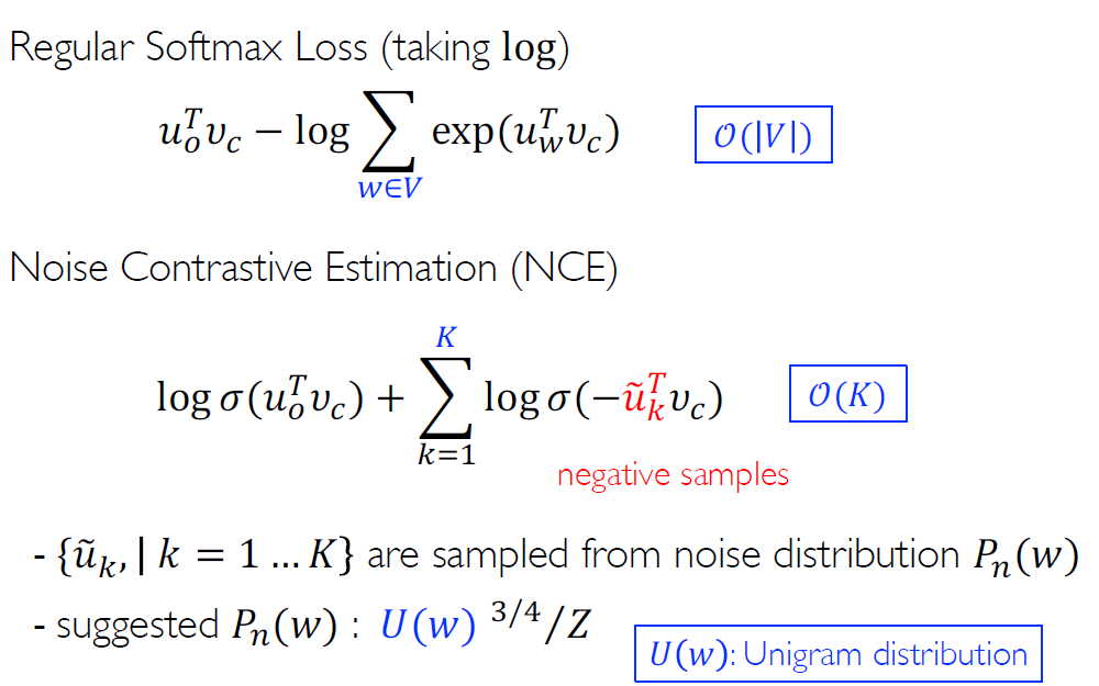
NCE is essentially an approximation of softmax (taking log), which converts the v-category problem into a bicategory problem. \(U(w)\) is the distribution of word frequency. We sample K words (negtive sampling) based on \(P_n(w)\) (using 3/4 as an exponential can reduce the impact of overly high frequency stop words on sampling). K often takes from 10~200.
Hierarchical softmax
The hierarchical softmax groups words by frequency with a Huffman tree, reduces the computation complexity of each step from 𝑉 to log𝑉.
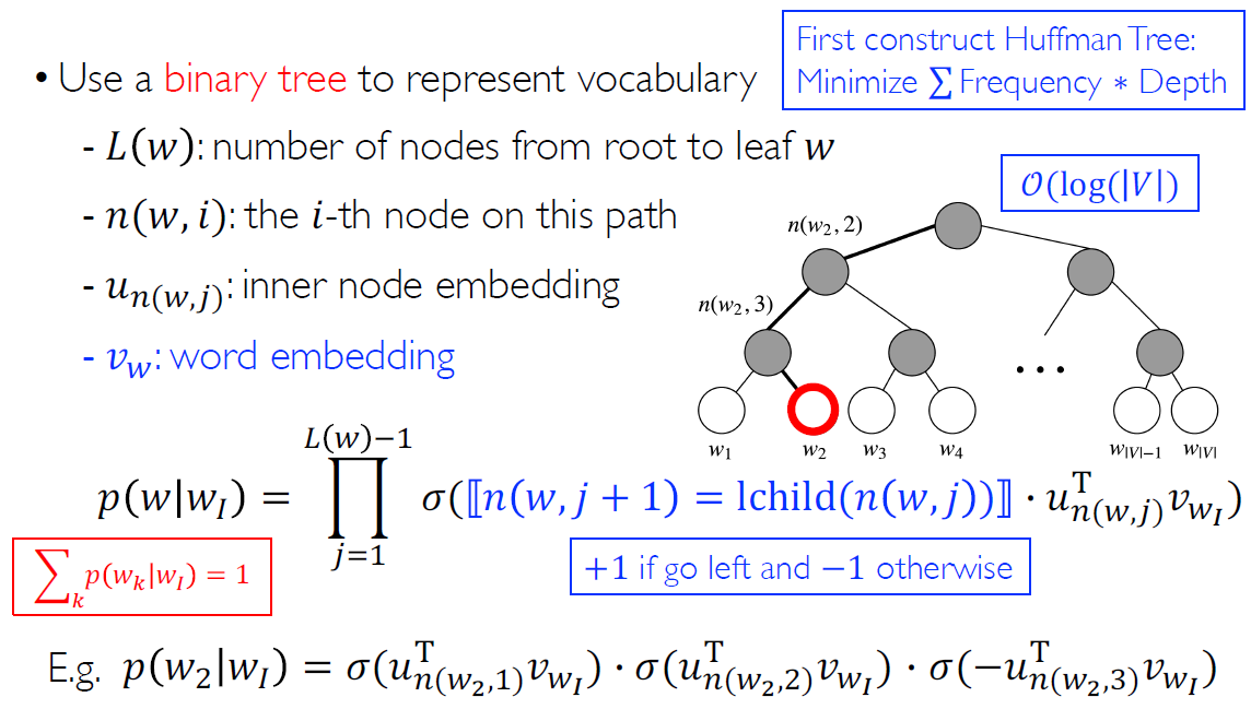
The leaves on the tree represent all the words in the vocabulary. We consider the process of calculating conditional probabilities as the softmax of dot product of node embedding and word embedding from root to leaf node. (\(w_I\) indicates the input word).
We consider the process of calculating the conditional probability as a serial multiplication of softmax of the vector product of each inner node embedding on the path from the root to the leaf corresponding to the target word. If it go left, the blue part of the formula get 1, else -1.
Beyond Word2vec
Subword Information: FastText
Word2vec assigns a distinct vector to each word, which ignores the internal structure of words, performs bad when vocabulary is large and some words are rare.
Therefore FastText uses subword to get word embedding. It firstly represent each word as a bag of character n-gram (e.g. 3-gram subword of where is { <wh, whe, her, ere, re>,
It can shares the representations across words, but it can also lead to increased complexity due to a larger vocabulary (thus hierarchical softmax is needed).
Global Word Embedding: Glove
All the machine learning models above only consider the words within a sliding window but ignore the global statistical information i.e. co-occurrence matrix \(X\).
Thus the purpose of Glove is producing a vector space with meaningful sub-structure while using global statistical information.
The original similarity between two word i and j which in context with each other is
Due to the denominator is computationally huge, so we discard the normalization and get an approximation
The original likelyhood function is
Glove transform it into a weighted version and taking log
where the weighting factor \(f\left(X_{i j}\right)\) is co-occurrence matrix \(X_{ij}\). The reason for taking logarithm is that \(X_{ij}\) is usually larger and difficult for optimization.

