Paper: Bidirectional LSTM-CRF Models for Sequence Tagging
Bidirectional LSTM-CRF Models for Sequence Tagging
abstract:
This paper systematically proposed four model, respectively named LSTM, LSTM+CRF, Bi-LSTM, Bi-LSTM+CRF.
Main part: The BI-LSTMCRF model can produce state of the art (or close to) accuracy on POS, chunking and NER data sets.
In addition, it is robust and has less dependence on word embedding as compared to previous observations.
1. Introduction:
Sequence tagging including part of speech tagging (POS), chunking, and named entity recognition (NER) has been a classic NLP task. It has drawn research attention for a few decades. The output of taggers can be used for down streaming applications.
Most existing sequence tagging models are linear statistical models which include:
- Hidden Markov Models (HMM)
- Maximum entropy Markov models (MEMMs) (McCallum et al., 2000)
- Conditional Random Fields (CRF)(Lafferty et al., 2001)
Convolutional network based models (Collobert et al., 2011) have been recently proposed to tackle sequence tagging problem. We denote such a model as Conv-CRF as it consists of a convolutional network and a CRF layer on the output (the term of sentence level loglikelihood (SSL) was used in the original paper). The Conv-CRF model has generated promising results on sequence tagging tasks.
In speech language understanding community, recurrent neural network (Mesnil et al., 2013; Yao et al., 2014) and convolutional nets (Xu and Sarikaya, 2013) based models have been recently proposed. Other relevant work includes (Graves et al., 2005; Graves et al., 2013) which proposed a bidirectional recurrent neural network for speech recognition.
In this paper, we propose a variety of neural network based models to sequence tagging task. These models include LSTM networks, bidirectional LSTM networks (BI-LSTM), LSTM networks with a CRF layer (LSTM-CRF), and bidirectional LSTM networks with a CRF layer (BILSTM-CRF). Our contributions can be summarized as follows.
1) We systematically compare the performance of aforementioned models on NLP tagging data sets;
2) Our work is the first to apply a bidirectional LSTM CRF (denoted as BI-LSTM-CRF) model to NLP benchmark sequence tagging data sets. This model can use both past and future input features thanks to a bidirectional LSTM component. In addition, this model can use sentence level tag information thanks to a CRF layer. Our model can produce state of the art (or close to) accuracy on POS, chunking and NER data sets;
3) We show that BI-LSTMCRF model is robust and it has less dependence on word embedding as compared to previous observations (Collobert et al., 2011). It can produce accurate tagging performance without resorting to word embedding.
2. Models:
In this section, we describe the models used in this paper: LSTM, BI-LSTM, CRF, LSTM-CRF and BI-LSTM-CRF.
RNN:
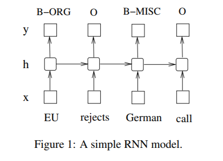
Figure 1 illustrates a named entity recognition system in which each word is tagged with other (O) or one of four entity types:
Person (PER), Location (LOC), Organization (ORG), and Miscellaneous (MISC). So, we have five taggers: PER, LOC, ORG, MISC, O
The sentence of EU rejects German call to boycott British lamb . is tagged as B-ORG O B-MISC O O O B-MISC O O, where B-, I- tags indicate beginning and intermediate positions of entities.
2.1 LSTM
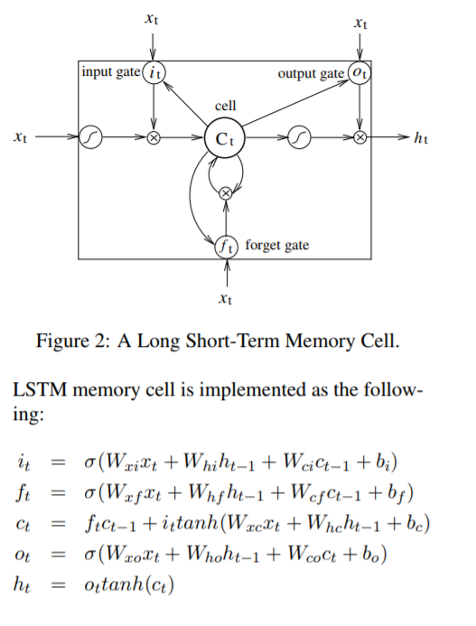
Fig. 3 shows a LSTM sequence tagging model which employs aforementioned LSTM memory cells (dashed boxes with rounded corners).

2.2 Bi-LSTM
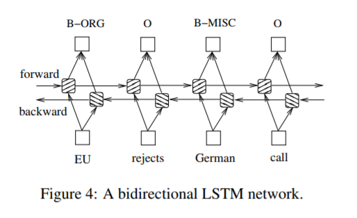
In sequence tagging task, we have access to both past and future input features for a given time, we can thus utilize a bidirectional LSTM network (Figure 4) as proposed in (Graves et al., 2013). In doing so, we can efficiently make use of past features (via forward states) and future features (via backward states) for a specific time frame.
We train bidirectional LSTM networks using backpropagation through time (BPTT)(Boden., 2002). The forward and backward passes over the unfolded network over time are carried out in a similar way to regular network forward and backward passes, except that we need to unfold the hidden states for all time steps.
We also need a special treatment at the beginning and the end of the data points. In our implementation, we do forward and backward for whole sentences and we only need to reset the hidden states to 0 at the begging of each sentence. We have batch implementation which enables multiple sentences to be processed at the same time.
2.3 CRF networks
There are two different ways to make use of neighbor tag information in predicting current tags:
- The first is to predict a distribution of tags for each time step and then use beam-like decoding to find optimal tag sequences. The work of maximum entropy classifier (Ratnaparkhi, 1996) and Maximum entropy Markov models (MEMMs) (McCallum et al., 2000) fall in this category.
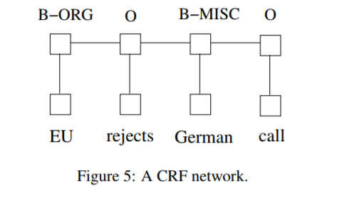
- The second one is to focus on sentence level instead of individual positions, thus leading to Conditional Random Fields (CRF) models (Lafferty et al., 2001) (Fig. 5). Note that the inputs and outputs are directly connected, as opposed to LSTM and bidirectional LSTM networks where memory cells/recurrent components are employed.
It has been shown that CRFs can produce higher tagging accuracy in general. It is interesting that the relation between these two ways of using tag information bears resemblance to two ways of using input features (see aforementioned LSTM and BI-LSTM networks), and the results in this paper confirms the superiority of BI-LSTM compared to LSTM.
2.4 LSTM-CRF networks
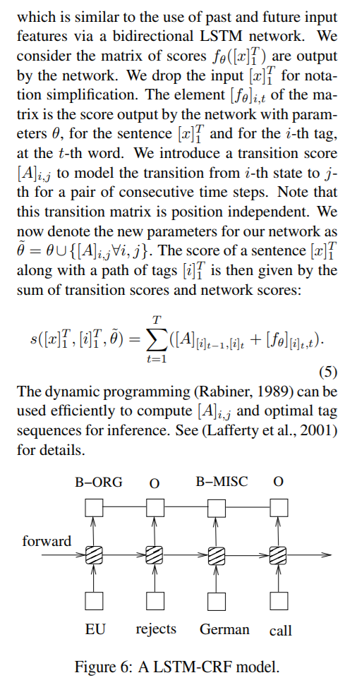
We combine a LSTM network and a CRF network to form a LSTM-CRF model, which is shown in Fig. 6. This network can efficiently use past input features via a LSTM layer and sentence level tag information via a CRF layer. A CRF layer is represented by lines which connect consecutive output layers. A CRF layer has a state transition matrix as parameters. With such a layer, we can efficiently use past and future tags to predict the current tag,
2.5 BI-LSTM-CRF networks
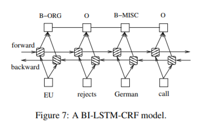
Similar to a LSTM-CRF network, we combine a bidirectional LSTM network and a CRF network to form a BI-LSTM-CRF network (Fig. 7). In addition to the past input features and sentence level tag information used in a LSTM-CRF model, a BILSTM-CRF model can use the future input features. The extra features can boost tagging accuracy as we will show in experiments.
3 Training procedure
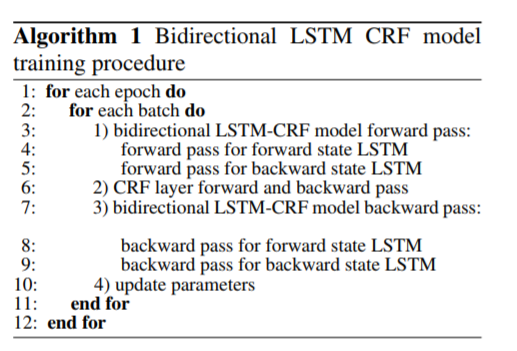
All models used in this paper share a generic SGD forward and backward training procedure. We choose the most complicated model, BI-LSTMCRF, to illustrate the training algorithm as shown in Algorithm 1. In each epoch, we divide the whole training data to batches and process one batch at a time. Each batch contains a list of sentences which is determined by the parameter of batch size. In our experiments, we use batch size of 100 which means to include sentences whose total length is no greater than 100. For each batch, we first run bidirectional LSTM-CRF model forward pass which includes the forward pass for both forward state and backward state of LSTM. As a result, we get the the output score fθ([x] T1 ) for all tags at all positions. We then run CRF layer forward and backward pass to compute gradients for network output and state transition edges. After that, we can back propagate the errors from the output to the input, which includes the backward pass for both forward and backward states of LSTM. Finally we update the network parameters which include the state transition matrix [A]i,j ∀i, j, and the original bidirectional LSTM parameters θ.
4 Experiments
4.1 Data
We test LSTM, BI-LSTM, CRF, LSTM-CRF, and BI-LSTM-CRF models on three NLP tagging tasks: Penn TreeBank (PTB) POS tagging, CoNLL 2000 chunking, and CoNLL 2003 named entity tagging. Table 1 shows the size of sentences, tokens, and labels for training, validation and test sets respectively. POS assigns each word with a unique tag that indicates its syntactic role. In chunking, each word is tagged with its phrase type. For example, tag B-NP indicates a word starting a noun phrase. In NER task, each word is tagged with other or one of four entity types: Person, Location, Organization, or Miscellaneous. We use the BIO2 annotation standard for chunking and NER tasks.
4.2 Features
We extract the same types of features for three data sets. The features can be grouped as spelling features and context features. As a result, we have 401K, 76K, and 341K features extracted for POS, chunking and NER data sets respectively. These features are similar to the features extracted from Stanford NER tool (Finkel et al., 2005; Wang and Manning, 2013). Note that we did not use extra data for POS and chunking tasks, with the exception of using Senna embedding (see Section 4.2.3). For NER task, we report performance with spelling and context features, and also incrementally with Senna embedding and Gazetteer features1 .
4.3 OMIT


