拓端tecdat|R语言广义线性模型GLM、多项式回归和广义可加模型GAM预测泰坦尼克号幸存者

原文链接：http://tecdat.cn/?p=18266

 

本文通过R语言建立广义线性模型(GLM)、多项式回归和广义可加模型（GAM）来预测谁在1912年的泰坦尼克号沉没中幸存下来。

1.  
    
2.  
   str(titanic)

数据变量为：

• Survived：乘客存活指标（如果存活则为1）
• Pclass：旅客舱位等级
• Sex：乘客性别
• Age：乘客年龄
• SibSp：兄弟姐妹/配偶人数
• Parch：父母/子女人数
• Embarked： 登船港口
• Name：旅客姓名

最后一个变量使用不多，因此我们将其删除，

titanic = titanic[,1:7]

现在，我们回答问题：

幸存的旅客比例是多少？

简单的答案是

 

1.  
   mean(titanic$Survived)
2.  
   [1] 0.3838384

可以在下面的列联表中找到

1.  
   table(titanic$Survived)/nrow(titanic)
2.  
   0 1
3.  
   0.6161616 0.3838384

或此处幸存者的38.38 ％。也就是说，也可以通过不对任何解释变量进行逻辑回归来获得（换句话说，仅对常数进行回归）。回归给出了：

1.  
    
2.  
   Coefficients:
3.  
   (Intercept)
4.  
   -0.4733
5.  
    
6.  
   Degrees of Freedom: 890 Total (i.e. Null); 890 Residual
7.  
   Null Deviance: 1187
8.  
   Residual Deviance: 1187 AIC: 1189

给出β0的值，并且由于生存概率为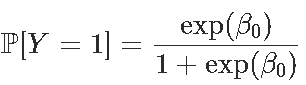

我们通过考虑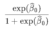

 

1.  
   exp(-0.4733)/(1+exp(-0.4733))
2.  
   [1] 0.3838355

我们也可以使用predict函数 

1.  
   predict(glm(Survived~1, family=binomial,type="response")[1]
2.  
   1
3.  
   0.3838384

此外，在概率回归中也适用，

1.  
   reg=glm(Survived~1, family=binomial(link="probit"),data=titanic)
2.  
   predict(reg,type="response")[1]
3.  
   1
4.  
   0.3838384

幸存的头等舱乘客的比例是多少？

我们只看头等舱的人，

 

[1] 0.6296296

约63％存活。我们可以进行逻辑回归

1.  
    
2.  
   Coefficients:
3.  
   (Intercept) Pclass2 Pclass3
4.  
   0.5306 -0.6394 -1.6704
5.  
    
6.  
   Degrees of Freedom: 890 Total (i.e. Null); 888 Residual
7.  
   Null Deviance: 1187
8.  
   Residual Deviance: 1083 AIC: 1089

由于第1类是参考类，因此我们照旧考虑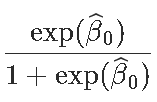

1.  
   exp(0.5306)/(1+exp(0.5306))
2.  
   [1] 0.629623

predict预测：

1.  
    
2.  
   predict(reg,newdata=data.frame(Pclass="1"),type="response")
3.  
   1
4.  
   0.6296296

我们可以尝试概率回归，我们得到的结果是一样的，

1.  
    
2.  
   predict(reg,newdata=data.frame(Pclass="1"),type="response")
3.  
   1
4.  
   0.6296296

卡方独立性测试 ：在生存与否之间的检验统计量是多少？

卡方检验的命令如下

1.  
   chisq.test(table( Survived, Pclass))
2.  
    
3.  
   Pearson's Chi-squared test
4.  
    
5.  
   data: table( Survived, Pclass)
6.  
   X-squared = 102.89, df = 2, p-value < 2.2e-16

我们有一个列联表，如果变量是独立的，我们有，然后是统计量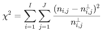，我们可以看到，对测试的贡献

1.  
    
2.  
   1 2 3
3.  
   0 -4.601993 -1.537771 3.993703
4.  
   1 5.830678 1.948340 -5.059981

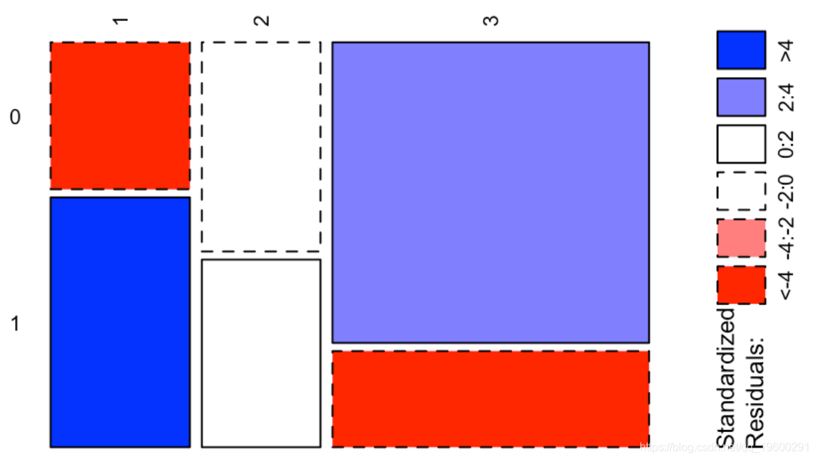
这给了我们很多信息：我们观察到两个正值，分别对应于“幸存”和“头等舱”与“无法幸存”和“三等舱”之间的强（正）关联，以及两个很强的负值，对应于“生存”和“第三等”之间的强烈负相关，以及“无法幸存”和“头等舱”。我们可以在下图上可视化这些值

 

 

1.  
    
2.  
   ass(table( Survived, Pclass), shade = TRUE, las=3)

 

然后我们必须进行逻辑回归，并预测两名模拟乘客的生存概率

假设我们有两名乘客

1.  
   newbase = data.frame(
2.  
   Pclass = as.factor(c(1,3)),
3.  
   Sex = as.factor(c("female","male")),
4.  
   Age = c(17,20),
5.  
   SibSp = c(1,0),
6.  
   Parch = c(2,0),

让我们对所有变量进行简单回归，

1.  
    
2.  
    
3.  
   Coefficients:
4.  
   Estimate Std. Error z value Pr(>|z|)
5.  
   (Intercept) 16.830381 607.655774 0.028 0.97790
6.  
   Pclass2 -1.268362 0.298428 -4.250 2.14e-05 ***
7.  
   Pclass3 -2.493756 0.296219 -8.419 < 2e-16 ***
8.  
   Sexmale -2.641145 0.222801 -11.854 < 2e-16 ***
9.  
   Age -0.043725 0.008294 -5.272 1.35e-07 ***
10.  
    SibSp -0.355755 0.128529 -2.768 0.00564 **
11.  
    Parch -0.044628 0.120705 -0.370 0.71159
12.  
    EmbarkedC -12.260112 607.655693 -0.020 0.98390
13.  
    EmbarkedQ -13.104581 607.655894 -0.022 0.98279
14.  
    EmbarkedS -12.687791 607.655674 -0.021 0.98334
15.  
    ---
16.  
    Signif. codes: 0 ‘***’ 0.001 ‘**’ 0.01 ‘*’ 0.05 ‘.’ 0.1 ‘ ’ 1
17.  
     
18.  
    (Dispersion parameter for binomial family taken to be 1)
19.  
     
20.  
    Null deviance: 964.52 on 713 degrees of freedom
21.  
    Residual deviance: 632.67 on 704 degrees of freedom
22.  
    (177 observations deleted due to missingness)
23.  
    AIC: 652.67
24.  
     
25.  
    Number of Fisher Scoring iterations: 13

两个变量并不重要。我们删除它们

1.  
    
2.  
    
3.  
   Coefficients:
4.  
   Estimate Std. Error z value Pr(>|z|)
5.  
   (Intercept) 4.334201 0.450700 9.617 < 2e-16 ***
6.  
   Pclass2 -1.414360 0.284727 -4.967 6.78e-07 ***
7.  
   Pclass3 -2.652618 0.285832 -9.280 < 2e-16 ***
8.  
   Sexmale -2.627679 0.214771 -12.235 < 2e-16 ***
9.  
   Age -0.044760 0.008225 -5.442 5.27e-08 ***
10.  
    SibSp -0.380190 0.121516 -3.129 0.00176 **
11.  
    ---
12.  
    Signif. codes: 0 ‘***’ 0.001 ‘**’ 0.01 ‘*’ 0.05 ‘.’ 0.1 ‘ ’ 1
13.  
     
14.  
    (Dispersion parameter for binomial family taken to be 1)
15.  
     
16.  
    Null deviance: 964.52 on 713 degrees of freedom
17.  
    Residual deviance: 636.56 on 708 degrees of freedom
18.  
    (177 observations deleted due to missingness)
19.  
    AIC: 648.56
20.  
     
21.  
    Number of Fisher Scoring iterations: 5

我们有年龄这样的连续变量时，我们可以进行多项式回归

1.  
    
2.  
    
3.  
   Coefficients:
4.  
   Estimate Std. Error z value Pr(>|z|)
5.  
   (Intercept) 3.0213 0.2903 10.408 < 2e-16 ***
6.  
   Pclass2 -1.3603 0.2842 -4.786 1.70e-06 ***
7.  
   Pclass3 -2.5569 0.2853 -8.962 < 2e-16 ***
8.  
   Sexmale -2.6582 0.2176 -12.216 < 2e-16 ***
9.  
   poly(Age, 3)1 -17.7668 3.2583 -5.453 4.96e-08 ***
10.  
    poly(Age, 3)2 6.0044 3.0021 2.000 0.045491 *
11.  
    poly(Age, 3)3 -5.9181 3.0992 -1.910 0.056188 .
12.  
    SibSp -0.5041 0.1317 -3.828 0.000129 ***
13.  
    ---
14.  
    Signif. codes: 0 ‘***’ 0.001 ‘**’ 0.01 ‘*’ 0.05 ‘.’ 0.1 ‘ ’ 1
15.  
     
16.  
    (Dispersion parameter for binomial family taken to be 1)
17.  
     
18.  
    Null deviance: 964.52 on 713 degrees of freedom
19.  
    Residual deviance: 627.55 on 706 degrees of freedom
20.  
    AIC: 643.55
21.  
     
22.  
    Number of Fisher Scoring iterations: 5

但是解释参数变得很复杂。我们注意到三阶项在这里很重要，因此我们将手动进行回归

1.  
    
2.  
   Coefficients:
3.  
   Estimate Std. Error z value Pr(>|z|)
4.  
   (Intercept) 5.616e+00 6.565e-01 8.554 < 2e-16 ***
5.  
   Pclass2 -1.360e+00 2.842e-01 -4.786 1.7e-06 ***
6.  
   Pclass3 -2.557e+00 2.853e-01 -8.962 < 2e-16 ***
7.  
   Sexmale -2.658e+00 2.176e-01 -12.216 < 2e-16 ***
8.  
   Age -1.905e-01 5.528e-02 -3.446 0.000569 ***
9.  
   I(Age^2) 4.290e-03 1.854e-03 2.314 0.020669 *
10.  
    I(Age^3) -3.520e-05 1.843e-05 -1.910 0.056188 .
11.  
    SibSp -5.041e-01 1.317e-01 -3.828 0.000129 ***
12.  
    ---
13.  
    Signif. codes: 0 ‘***’ 0.001 ‘**’ 0.01 ‘*’ 0.05 ‘.’ 0.1 ‘ ’ 1
14.  
     
15.  
    (Dispersion parameter for binomial family taken to be 1)
16.  
     
17.  
    Null deviance: 964.52 on 713 degrees of freedom
18.  
    Residual deviance: 627.55 on 706 degrees of freedom
19.  
    AIC: 643.55
20.  
     
21.  
    Number of Fisher Scoring iterations: 5

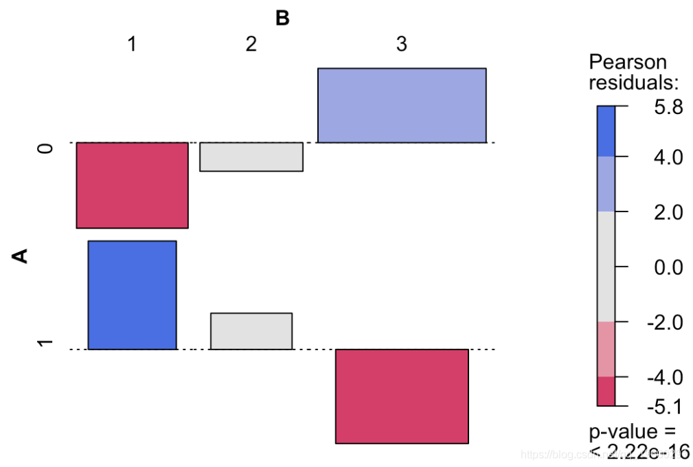
可以看到，p值是相同的。简而言之，将年龄转换为年龄的非线性函数是有意义的。可以可视化此函数

1.  
    
2.  
   plot(xage,yage,xlab="Age",ylab="",type="l")

 

实际上，我们可以使用样条曲线。广义可加模型（ gam ）是完美的可视化工具

1.  
    
2.  
    
3.  
   (Dispersion Parameter for binomial family taken to be 1)
4.  
    
5.  
   Null Deviance: 964.516 on 713 degrees of freedom
6.  
   Residual Deviance: 627.5525 on 706 degrees of freedom
7.  
   AIC: 643.5525
8.  
   177 observations deleted due to missingness
9.  
    
10.  
    Number of Local Scoring Iterations: 4
11.  
     
12.  
    Anova for Parametric Effects
13.  
    Df Sum Sq Mean Sq F value Pr(>F)
14.  
    Pclass 2 26.72 13.361 11.3500 1.407e-05 ***
15.  
    Sex 1 131.57 131.573 111.7678 < 2.2e-16 ***
16.  
    bs(Age) 3 22.76 7.588 6.4455 0.0002620 ***
17.  
    SibSp 1 14.66 14.659 12.4525 0.0004445 ***
18.  
    Residuals 706 831.10 1.177
19.  
    ---
20.  
    Signif. codes: 0 ‘***’ 0.001 ‘**’ 0.01 ‘*’ 0.05 ‘.’ 0.1 ‘ ’ 1

我们可以看到年龄变量的变换，

 

并且我们发现变换接近于我们的3阶多项式。我们可以添加置信带，从而可以验证该函数不是真正的线性

 

我们现在有三个模型。最后给出了两个模拟乘客的预测，

1.  
   predict(reg,newdata=newbase,type="response")
2.  
   1 2
3.  
   0.9605736 0.1368988
4.  
   predict(reg3,newdata=newbase,type="response")
5.  
   1 2
6.  
   0.9497834 0.1218426
7.  
   predict(regam,newdata=newbase,type="response")
8.  
   1 2
9.  
   0.9497834 0.1218426

可以看到莱昂纳多·迪卡普里奥（  Leonardo DiCaprio） 有大约12％的幸存机会（考虑到他的年龄，他有三等票，而且船上没有家人）。

---

最受欢迎的见解

1.用SPSS估计HLM层次线性模型模型

2.R语言线性判别分析（LDA），二次判别分析（QDA）和正则判别分析（RDA）

3.基于R语言的lmer混合线性回归模型

4.R语言Gibbs抽样的贝叶斯简单线性回归仿真分析

5.在r语言中使用GAM（广义相加模型）进行电力负荷时间序列分析

6.使用SAS，Stata，HLM，R，SPSS和Mplus的分层线性模型HLM

7.R语言中的岭回归、套索回归、主成分回归：线性模型选择和正则化

8.R语言用线性回归模型预测空气质量臭氧数据

9.R语言分层线性模型案例