拓端tecdat|R语言代写使用Metropolis- Hasting抽样算法进行逻辑回归

在逻辑回归中，我们将二元响应\（Y_i \）回归到协变量\（X_i \）上。下面的代码使用Metropolis采样来探索\（\ beta_1 \）和\（\ beta_2 \）的后验YiYi到协变量XiXi。让

定义expit和分对数链接函数

 logit<-function(x){log(x/(1-x))} 此函数计算\（（\ beta_1，\ beta_2）\）的联合后验。它返回后验的对数以获得数值稳定性。(β1,β2)(β1,β2)。它返回后验的对数以获得数值稳定性。

log_post<-function(Y,X,beta){
    prob1  <- expit(beta[1] + beta[2]*X)
     prior  <- sum(dnorm(beta,0,10,log=TRUE))
like+prior}

这是MCMC的主要功能.can.sd是候选标准偏差。

Bayes.logistic<-function(y,X,
                         n.samples=10000,
                         can.sd=0.1){
 
     keep.beta     <- matrix(0,n.samples,2)
     keep.beta[1,] <- beta

     acc   <- att <- rep(0,2)
 
    for(i in 2:n.samples){

      for(j in 1:2){

       att[j] <- att[j] + 1

      # Draw candidate:

       canbeta    <- beta
       canbeta[j] <- rnorm(1,beta[j],can.sd)
       canlp      <- log_post(Y,X,canbeta)

      # Compute acceptance ratio:

       R <- exp(canlp-curlp)  
       U <- runif(1)                          
       if(U<R){       
         beta   <- canbeta
          acc[j] <- acc[j]+1
       }
     }
     keep.beta[i,]<-beta

   }
   # Return the posterior samples of beta and
   # the Metropolis acceptance rates
list(beta=keep.beta,acc.rate=acc/att)}

生成一些模拟数据

 set.seed(2008)
 n         <- 100
 X         <- rnorm(n)
  true.p    <- expit(true.beta[1]+true.beta[2]*X)
 Y         <- rbinom(n,1,true.p)

适合模型

 burn      <- 10000
 n.samples <- 50000
  fit  <- Bayes.logistic(Y,X,n.samples=n.samples,can.sd=0.5)
 tock <- proc.time()[3]

 tock-tick

## elapsed 
##    3.72

结果

 fit$acc.rate # Acceptance rates

## [1] 0.4504290 0.5147703

 acf(fit$beta)

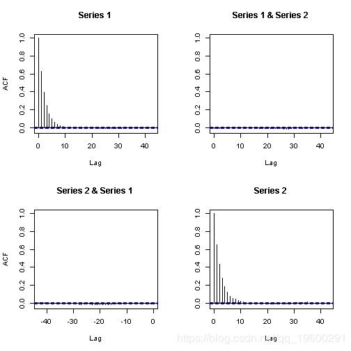
  abline(true.beta[1],0,lwd=2,col=2)

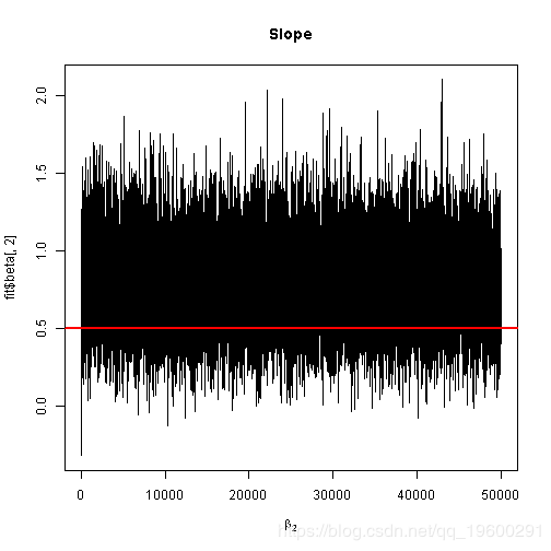
  abline(true.beta[2],0,lwd=2,col=2)

 hist(fit$beta[,1],main="Intercept",xlab=expression(beta[1]),breaks=50)

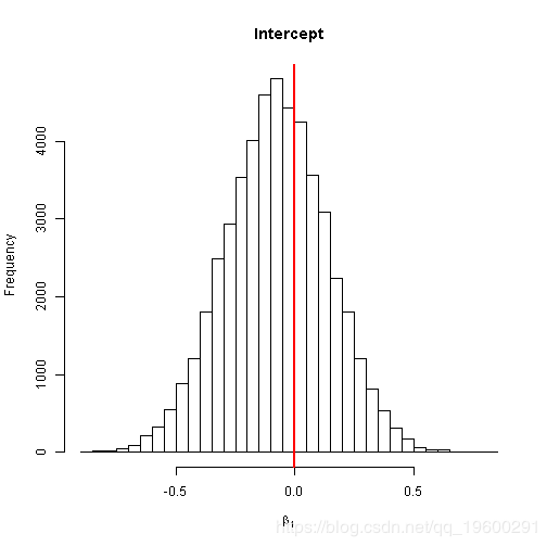
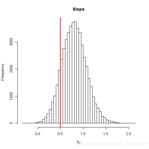
 hist(fit$beta[,2],main="Slope",xlab=expression(beta[2]),breaks=50)
 abline(v=true.beta[2],lwd=2,col=2)

 print("Posterior mean/sd")

## [1] "Posterior mean/sd"

 print(round(apply(fit$beta[burn:n.samples,],2,mean),3))

## [1] -0.076  0.798

 print(round(apply(fit$beta[burn:n.samples,],2,sd),3))

## [1] 0.214 0.268

    print(summary(glm(Y~X,family="binomial")))

## 
## Call:
## glm(formula = Y ~ X, family = "binomial")
## 
## Deviance Residuals: 
##     Min       1Q   Median       3Q      Max  
## -1.6990  -1.1039  -0.6138   1.0955   1.8275  
## 
## Coefficients:
##             Estimate Std. Error z value Pr(>|z|)   
## (Intercept) -0.07393    0.21034  -0.352  0.72521   
## X            0.76807    0.26370   2.913  0.00358 **
## ---
## Signif. codes:  0 '***' 0.001 '**' 0.01 '*' 0.05 '.' 0.1 ' ' 1
## 
## (Dispersion parameter for binomial family taken to be 1)
## 
##     Null deviance: 138.47  on 99  degrees of freedom
## Residual deviance: 128.57  on 98  degrees of freedom
## AIC: 132.57
## 
## Number of Fisher Scoring iterations: 4