四元数基础（二）

 

　　有了一些四元数的基础后，我们再继续挖点东西出来。这一节，我们来讨论一下四元数的指数映射，对数映射，球面插值等内容。

指数映射

　　首先，我们定义一般四元数的指数映射为：$$e^{\mathbf{q}} = \sum_{k=0}^{\infty}{\frac{1}{k!}\mathbf{q}^k}$$ 其中， $\mathbf{q}^k$表示$k$个相同四元数$\mathbf{q}$的 $\otimes$ 累乘。不难发现，一个四元数的指数映射仍然是一个四元数。有了这个定义后，我们来关注一下纯虚四元数的指数映射，令 $\mathbf{v} = v_x i + v_y j + v_z k$ 为一个纯虚四元数，我们总可以把一个纯虚四元数写成如下形式：$$\mathbf{v} = \theta \mathbf{u}$$ 其中，$\mathbf{u}$ 是单位纯虚四元数，而 $\theta = \| \mathbf{v} \| \in \mathbb{R}$。 接着，我们把这个纯虚四元数做一个指数映射： $$e^{\mathbf{v}} = e^{\theta \mathbf{u}} = \left(1-\frac{\theta ^ 2}{2!} + \frac{\theta ^4}{4!} + ...\right) + \left( \mathbf{u}\theta -  \mathbf{u} \frac{\theta^3}{3!} + \mathbf{u} \frac{\theta^5}{5!} + ... \right)$$ 需要说明一下的是，上式第二个大括号中简洁的结果利用了 $\mathbf{u} \otimes \mathbf{u} = -1$ 这一结果。两个大括号内的内容，咋一看怎么都非常熟悉。没错！他们刚好分别是$\cos \theta$ 和 $\sin \theta$ 的泰勒展开式。因此，一个纯虚四元数的指数映射结果变得就非常简洁了： $$e^{\mathbf{v}} =  e^{\theta \mathbf{u}} = \cos \theta + \mathbf{u} \sin \theta = \left [ \begin{array}  {*{20}{c}} \cos \theta \\ \mathbf{u} \sin \theta \end{array} \right] = \left [ \begin{array}  {*{20}{c}} \cos \theta \\ u_x \sin \theta \\  u_y \sin \theta \\ u_z \sin \theta \end{array} \right] $$ 如果你学过复变函数，那么这个式子的形式你应该会非常眼熟，因为它和欧拉公式 $e^{i\theta} = \cos \theta + i \sin \theta$ 简直太像了！ 注意到， $\| e^{\mathbf{v}} \|  = \cos^2 \theta +\sin ^2 \theta = 1$。 因此，一个纯虚四元数经过指数映射后得到的是单位四元数！提到单位四元数，你脑中必须想到的就是 “旋转” 二字。另外，我们知道对于单位四元数来说，它的逆和共轭是相等的，因此：$$e^{-\mathbf{v}} = \left( e^{\mathbf{v}} \right) ^ *$$

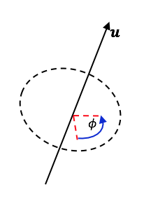
　　现在，让我们回到旋转这个正题上来，看了这么多公式，你一定困惑：四元数如此抽象，如果给了一个单位四元数，我怎么知道它朝着什么方向转动了多少角度？既然要直观，我们首先把最直观的旋转向量搬出来。旋转向量直观的理解就是物体绕着一个固定轴旋转了多少角度，那我们记这个固定轴的单位方向向量为 $\mathbf{u}$ （三维向量，两个自由度），转动角度为$\phi$ （标量，一个自由度）。那么，一个旋转就可以用 $\phi \mathbf{u}$ 来表达。这样够直观了吧？还不够？来个图：　

 

 

　　好，假设你现在理解了旋转向量。那接下来你就可能会问：单位四元数和旋转向量有什么关系呢？我把结果直接列在这里：$$\mathbf{q} = \text{Exp} (\phi \mathbf{u}) = e^{\phi \mathbf{u} / 2} = \cos \frac{\phi}{2} + \mathbf{u} \sin \frac{\phi}{2} = \left [ \begin{array}  {*{20}{c}} \cos (\phi /2 ) \\ \mathbf{u} \sin (\phi/2) \end{array} \right] = \left [ \begin{array}  {*{20}{c}} \cos \frac{\phi}{2} \\ u_x \sin \frac{\phi}{2} \\  u_y \sin \frac{\phi}{2} \\ u_z \sin \frac{\phi}{2} \end{array} \right] $$

　　Note: 这里引入了记号 $\text{Exp}(\cdot)$，它和 $\exp{(\cdot)}$ 的关系是：$$\text{Exp}(\mathbf{v}) =\exp(\mathbf{v}/2) = e^{\mathbf{v}/2} $$ 两者其实并无本质无别，只是映射向量有没有除以2这一区别，但不论有没有除以2，三维向量用四元数来表示的话，它都是一个纯虚的四元数。因此，经过指数映射后，我们会得到一个单位四元数。

　　反过来，已知一个抽象的单位四元数 $\mathbf{q} = q_w + \mathbf{q}_v$，去得到对应的旋转向量就比较简单了： 

\begin{equation*}
\left\{
\begin{array}{lr}
\phi = 2\arccos(q_w) & \\
 \mathbf{u} =  \mathbf{q}_v / \sin (\phi / 2)
\end{array}
\right.
\end{equation*}

　　再来看一个有趣的现象，如果旋转角度 $\phi$ 加上 $2\pi$，旋转本身并没有变化，但是对应的四元数变成了 $-\mathbf{q}$。因此，任意两个互为相反数的单位四元数均可以表示同一个旋转。

　　现在，假设我们有一个三维空间点 $\mathbf{x}$，如果我们绕着 $\mathbf{u}$ 轴旋转 $\phi$ 角度，那么旋转后得到的点 $\mathbf{x}'$ 可以表达为： $$\mathbf{x}' = \mathbf{q} \otimes \mathbf{x} \otimes \mathbf{q}^*$$ 其中，$\mathbf{q} = \text{Exp}(\phi \mathbf{u})$，而三维空间点 $\mathbf{x}$ 在上式中被写成了纯虚四元数形式：$$\mathbf{x} = xi+yj+zk = \left [ \begin{array}  {*{20}{c}} 0 \\ \mathbf{x} \end{array} \right] \in \mathbb{H}_p$$ 为了方便记忆，我们姑且叫这个公式为三明治公式吧！请自行验证，三明治公式的结果一定是一个纯虚的四元数。否则，一个三维空间点或者说矢量经过旋转都不是一个点或者说矢量了，你说对么？　

对数映射

　　对数运算就是指数运算的逆运算。因此，把一个单位四元数 $\mathbf{q} = \cos (\phi /2) + \mathbf{u} \sin (\phi /2)$ （一个单位四元数总可以写成这种形式，这里为了让式子意义更加明确，把单位四元数用了它对应的旋转向量的轴 $\mathbf{u}$ 和角度 $\phi$ 来进行表达）进行对数映射，我们可以得到一个纯虚四元数，或者说一个3维向量：$$ \log(\mathbf{q}) = \log (\cos (\phi /2) + \mathbf{u} \sin (\phi /2)) = \log (e^{\mathbf{u} \phi/2}) = \mathbf{u} \phi/2$$ 为了和指数映射的 $\text{Exp}(\cdot)$ 保持一致，这里引入对数映射 $\text{Log}(\cdot)$，它和 $\log(\cdot)$的关系是： $$\text{Log}(\mathbf{q}) = 2\log{\mathbf{q}} = 2 \log (e^{\mathbf{u} \phi/2}) = \mathbf{u} \phi$$  

插值

• 方法一
  这里讨论的插值仅仅以单位四元数为对象。首先搞清楚问题是什么：给定两个旋转 $\mathbf{q}_0$ 和 $\mathbf{q}_1$ （再次强调：这必须是单位四元数！），我们期望当参数 $t$ 从0变到1的时候，我们找到的旋转也能“线性平稳”地从$\mathbf{q}_0$过渡到$\mathbf{q}_1$。假设我们记这个从$\mathbf{q}_0$到$\mathbf{q}_1$的旋转增量为$\Delta \mathbf{ q}$，使得：$$\mathbf{q}_1 = \mathbf{q}_0 \otimes \Delta \mathbf{q}$$ 对上面的等式，我们两边同时左乘以 $\mathbf{q}_{0}^{*}$，就可以得到：$$\Delta \mathbf{q} = \mathbf{q}_{0}^{*} \otimes \mathbf{q}_1 $$ 假设这个$\Delta \mathbf{ q}$对应的旋转角度为$\Delta \phi$，转轴为$\mathbf{ u}$，我们来看看$(\Delta \mathbf{ q})^t$ 这是个什么鬼？$$(\Delta \mathbf{ q})^t = \text{Exp}(\text{Log}(\Delta \mathbf{ q})^t) = \text{Exp}(t\text{Log}(\Delta \mathbf{ q})) $$ 另一方面，$\text{Log}(\Delta \mathbf{ q}) = \mathbf{u} \Delta \phi$，因此：$$(\Delta \mathbf{ q})^t = \text{Exp}((t\Delta \phi) \mathbf{u})$$ 咦，这刚刚好诶！角度变成了$t\Delta \phi$，当$t$从0变到1的时候，旋转角度能“线性”的过渡。同时，转轴不变，始终都是$\mathbf{u}$，也能满足我们的“平稳”要求。那么，就是它了，给定参数$t \in [0, 1]$，当$\mathbf{q}(t)$ 满足以下形式时，我们找到的旋转能线性平稳地从$\mathbf{q}_0$过渡到$\mathbf{q}_1$：$$\mathbf{q}(t) = \mathbf{q}_0 \otimes (\Delta \mathbf{q})^{t} = \mathbf{q}_0 \otimes (\mathbf{q}_{0}^{*} \otimes \mathbf{q}_1)^t$$ 当$t = 0$时，$\mathbf{q}(t) = \mathbf{q}(0) =   \mathbf{q}_0$，当 $t = 1$时，$\mathbf{q}(t) = \mathbf{q}(1) =   \mathbf{q}_0 \otimes \mathbf{q}_{0}^{*} \otimes \mathbf{q}_1 = \mathbf{q}_1$，完美！实际使用的话，我们采用下面的形式：$$\mathbf{q}(t) = \mathbf{q}_0 \otimes \left [ \begin{array}  {*{20}{c}} \cos (t \Delta \phi /2 ) \\ \mathbf{u} \sin (t \Delta \phi/2) \end{array} \right] $$ 总结一下：这种插值方法需要先计算旋转增量$\Delta \mathbf{ q}$，然后根据它计算所对应的轴 $\mathbf{ u}$ 以及旋转角度 $\Delta \phi$，再做四元数乘法去进行插值。
• 方法二
  这里给出另一种插值方法，称为球面插值公式，具体推导这里就不写了，有兴趣可以翻翻资料：$$\mathbf{q}(t) = \mathbf{q}_0 \frac{\sin((1-t)\Delta \theta)}{\sin(\Delta \theta)} + \mathbf{q}_1 \frac{\sin(t\Delta \theta) }{\sin(\Delta \theta)}$$ 其中，$\Delta \theta = \arccos(\mathbf{q}_{0}^{T}\mathbf{q}_1)$。 不难验证当$t = 0$时，$\mathbf{q}(t) = \mathbf{q}(0) =   \mathbf{q}_0$，当$t = 1$时，$\mathbf{q}(t) = \mathbf{q}(1) =   \mathbf{q}_1$。

　　

代码实例

　　下面采用Eigen库进行一些实际操练：

#include <iostream>
#include <Eigen/Dense>

int main()
{
    //arbitrary quaternion
    Eigen::Quaterniond Q(1, 3, 2, 5);
    std::cout << "(" << Q.w() << ", " << Q.x() << ", " << Q.y() << ", " << Q.z() << ")"<< std::endl;
    std::cout << Q.coeffs().transpose() << std::endl; //real part is at the end
    std::cout << Q.norm() << std::endl;

    Eigen::Quaterniond P = Q.conjugate();
    std::cout << "(" << P.w() << ", " << P.x() << ", " << P.y() << ", " << P.z() << ")"<< std::endl;
    Q.normalize();  //now can represent a rotation
    std::cout << "(" << Q.w() << ", " << Q.x() << ", " << Q.y() << ", " << Q.z() << ")"<< std::endl;



    //rotation quaternion -- unit quaternion
    double phi = M_PI / 3;  //rotation angle
    Eigen::Vector3d vec(1, 2, 3); //rotation vector
    vec.normalize();
    //method 1:
    Eigen::Quaterniond q1(cos(phi/2), vec(0) * sin(phi/2), vec(1) * sin(phi /2), vec(2) * sin(phi/2));
    //method 2:
    Eigen::Quaterniond q2(Eigen::AngleAxisd(phi, vec)); //a simple constructor
    //output
    std::cout << "(" << q1.w() << ", " << q1.x() << ", " << q1.y() << ", " << q1.z() << ")"<< std::endl;
    std::cout << "(" << q2.w() << ", " << q2.x() << ", " << q2.y() << ", " << q2.z() << ")"<< std::endl;
    //for unit quaternion, its inverse equals its conjugate
    Eigen::Quaterniond qConj = q1.conjugate();
    Eigen::Quaterniond qInv = q2.inverse();
    std::cout << "(" << qConj.w() << ", " << qConj.x() << ", " << qConj.y() << ", " << qConj.z() << ")"<< std::endl;
    std::cout << "(" << qInv.w() << ", " << qInv.x() << ", " << qInv.y() << ", " << qInv.z() << ")"<< std::endl;

    //from quaternion to rotation matrix
    Eigen::Matrix3d R1 = q1.matrix();
    Eigen::Matrix3d R2 = q2.toRotationMatrix();
    std::cout << "R1: \n" << R1 << std::endl << std::endl;
    std::cout << "R2: \n" << R2 << std::endl << std::endl;


    //quaternion product
    Eigen::Quaterniond p(2, 3, -1 ,5);
    Eigen::Quaterniond q(3,-1, 2, 4);
    p.normalize();
    q.normalize();
    Eigen::Quaterniond prod1 = p * q;
    std::cout << "(" << prod1.w() << ", " << prod1.x() << ", " << prod1.y() << ", " << prod1.z() << ")"<< std::endl;
    //calculate product using formula
    const double w = p.w() * q.w() - p.x() * q.x() - p.y() * q.y() - p.z() * q.z();
    const double x = p.w() * q.x() + p.x() * q.w() + p.y() * q.z() - p.z() * q.y();
    const double y = p.w() * q.y() - p.x() * q.z() + p.y() * q.w() + p.z() * q.x();
    const double z = p.w() * q.z() + p.x() * q.y() - p.y() * q.x() + p.z() * q.w();
    Eigen::Quaterniond prod2(w, x, y, z);
    std::cout << "(" << prod2.w() << ", " << prod2.x() << ", " << prod2.y() << ", " << prod2.z() << ")"<< std::endl;


    std::cout << "prod1---R: \n" << prod1.matrix() << std::endl;
    std::cout << "p.R * q.R \n" << p.matrix() * q.matrix() << std::endl;

    //rotate a point/vector via quaternion
    Eigen::Vector3d point(3, 4, 5);
    Eigen::Quaterniond point_quat(0, point(0), point(1), point(2)); //write into pure quaternion format
    Eigen::Quaterniond point_quat_rotated = p * point_quat * p.inverse();
    std::cout << "\n rotate a point/vector via quaternion: \n";
    std::cout << point_quat_rotated.coeffs().transpose() << std::endl;
    std::cout << p._transformVector(point).transpose() << std::endl; //an alternative way

    //rotate a point/vector via rotation matrix
    Eigen::Vector3d point_rotated = p.matrix() * point;
    std::cout << "\n rotate a point/vector via rotation martix: \n";
    std::cout << point_rotated.transpose() << std::endl << std::endl;


    //Interpolation
    Eigen::Quaterniond Q0(1, 3.1, 1.9, 4.2);
    Eigen::Quaterniond Q1(1.3, 2.7, 2.3, 4.1);
    Q0.normalize();
    Q1.normalize();
    const double t = 0.5;
    //Method 1:
    Eigen::Quaterniond dQ = Q0.inverse() * Q1;
    const double dPhi = 2 * acos(dQ.w());  //alternatively, Q0.angularDistance(Q1);
    Eigen::Vector3d u = Eigen::Vector3d(dQ.x(), dQ.y(), dQ.z()) / sin(dPhi * 0.5);
    Eigen::Quaterniond Qt1 = Q0 * Eigen::Quaterniond(cos(t*dPhi*0.5),
                                                    u(0)*sin(t*dPhi*0.5),
                                                    u(1)*sin(t*dPhi*0.5),
                                                    u(2) * sin(t*dPhi*0.5));
    Eigen::Quaterniond Qt2 = Q0 * Eigen::Quaterniond(Eigen::AngleAxisd(dPhi * t, u)); //another way to construct

    std::cout << "Q0: " << Q0.coeffs().transpose() << std::endl;
    std::cout << "Q1: " << Q1.coeffs().transpose() << std::endl;
    std::cout << "Q0.5 by method 1-1: " << Qt1.coeffs().transpose() << std::endl;
    std::cout << "Q0.5 by method 1-2: " << Qt2.coeffs().transpose() << std::endl;

    //Method 2:
    const double dTheta = acos(Q0.dot(Q1)); //alternatively, acos(Q0.coeffs().transpose() * Q1.coeffs());
    const double alpha = sin((1 - t) * dTheta) / sin(dTheta);
    const double beta = sin(t* dTheta) / sin(dTheta);
    Eigen::Quaterniond Qt3_1(Q0.w() * alpha, Q0.x() * alpha,
                             Q0.y() * alpha, Q0.z() * alpha);

    Eigen::Quaterniond Qt3_2 (Q1.w() * beta, Q1.x() * beta,
                              Q1.y() * beta, Q1.z() * beta);

    Eigen::Quaterniond Qt3(Qt3_1.w() + Qt3_2.w(),
                           Qt3_1.x() + Qt3_2.x(),
                           Qt3_1.y() + Qt3_2.y(),
                           Qt3_1.z() + Qt3_2.z());
    std::cout << "Q0.5 by method 2: " << Qt3.coeffs().transpose() << std::endl;

    //Method 3: call interface
    Eigen::Quaterniond Qt4 = Q0.slerp(t, Q1);
    std::cout << "Q0.5 by method 3: " << Qt4.coeffs().transpose() << std::endl;

    return  0;
}