神经网络介绍:梯度下降和正则化
一、梯度下降
梯度下降公式:$W^{[l]} = W^{[l]} - \alpha \text{ } dW^{[l]}$,$b^{[l]} = b^{[l]} - \alpha \text{ } db^{[l]}$,具体细节和代码实现参考文章神经网络介绍:算法基础
(Batch) Gradient Descent


### 伪代码
X = data_input
Y = labels
parameters = initialize_parameters(layers_dims)
for i in range(0, num_epochs):
    # Forward propagation
    a, caches = forward_propagation(X, parameters)
    # Compute cost.
    cost = compute_cost(a, Y)
    # Backward propagation.
    grads = backward_propagation(a, caches, parameters)
    # Update parameters.
    parameters = update_parameters(parameters, grads)
Stochastic Gradient Descent
### 伪代码
X = data_input
Y = labels
parameters = initialize_parameters(layers_dims)
for i in range(0, num_epochs):
    for j in range(0, m):
        # Forward propagation
        a, caches = forward_propagation(X[:,j], parameters)
        # Compute cost
        cost = compute_cost(a, Y[:,j])
        # Backward propagation
        grads = backward_propagation(a, caches, parameters)
        # Update parameters.
        parameters = update_parameters(parameters, grads)
Mini-Batch Gradient Descent
Mini-Batch Gradient Descent介于(Batch) Gradient Descent和Stochastic Gradient Descent之间,可分为两步进行:
- Build mini-batches from the training set (X, Y)
View Code
def random_mini_batches(X, Y, mini_batch_size = 64, seed = 0):
    """
    Creates a list of random minibatches from (X, Y)

    Arguments:
    X -- input data, of shape (number of features, number of examples)
    Y -- true label vector, of shape (1, number of examples)
    mini_batch_size -- size of the mini-batches, integer

    Returns:
    mini_batches -- list of synchronous (mini_batch_X, mini_batch_Y)
    """
    np.random.seed(seed)
    m = X.shape[1]   #number of training examples
    mini_batches = []
    # Step 1: Shuffle (X, Y)
    permutation = list(np.random.permutation(m))
    shuffled_X = X[:, permutation]
    shuffled_Y = Y[:, permutation].reshape((1,m))
    # Step 2: Partition (shuffled_X, shuffled_Y). Minus the end case.
    num_complete_minibatches = math.floor(m/mini_batch_size) # number of mini batches of size mini_batch_size
    for k in range(0, num_complete_minibatches):
        mini_batch_X = shuffled_X[:,k*mini_batch_size:(k+1)*mini_batch_size]
        mini_batch_Y = shuffled_Y[0,k*mini_batch_size:(k+1)*mini_batch_size].reshape((1,mini_batch_size))
        mini_batch = (mini_batch_X, mini_batch_Y)
        mini_batches.append(mini_batch)
    # Handling the end case (last mini-batch < mini_batch_size)
    if m % mini_batch_size != 0:
        mini_batch_X = shuffled_X[:,num_complete_minibatches*mini_batch_size:]
        mini_batch_Y = shuffled_Y[0,num_complete_minibatches*mini_batch_size:].reshape((1,m % mini_batch_size))
        mini_batch = (mini_batch_X, mini_batch_Y)
        mini_batches.append(mini_batch)
    return mini_batches
- Train the network
View Code
### 伪代码
X = data_input
Y = labels
parameters = initialize_parameters(layers_dims)
minibatches = random_mini_batches(X, Y)
for i in range(0, num_epochs):
    for minibatch in minibatches:
        # Select a minibatch
        (minibatch_X, minibatch_Y) = minibatch
        # Forward propagation
        a, caches = forward_propagation(minibatch_X, parameters)
        # Compute cost
        cost = compute_cost(a, minibatch_Y)
        # Backward propagation
        grads = backward_propagation(a, caches, parameters)
        # Update parameters.
        parameters = update_parameters(parameters, grads)
梯度下降、随机梯度下降与mini-batch梯度下降的区别在于进行一次参数更新所使用的训练样本数量。梯度下降一次更新需使用全部样本,计算效率较低;随机梯度下降一次更新仅使用一个样本,计算效率较高,但在过程中会产生较剧烈的震荡,影响最终的优化结果;mini-batch梯度下降则介于梯度下降和随机梯度下降两者之间,若选取合适的mini_batch_size,mini-batch梯度下降常优于梯度下降和随机梯度下降,特别是当训练数据集很大的情况下。
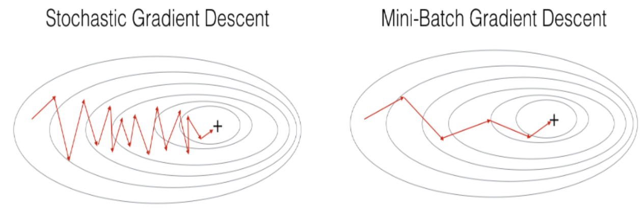
为进一步减少训练过程中不必要的震荡(如上图所示),加快收敛速度,并且尽可能地避免落入局部最优值,有一些改进的算法可供选择:
Momentum
$$ \begin{cases}
v_{dW^{[l]}} = \beta v_{dW^{[l]}} + (1 - \beta) dW^{[l]} \\
W^{[l]} = W^{[l]} - \alpha v_{dW^{[l]}}
\end{cases}\text{ and }\begin{cases}
v_{db^{[l]}} = \beta v_{db^{[l]}} + (1 - \beta) db^{[l]} \\
b^{[l]} = b^{[l]} - \alpha v_{db^{[l]}}
\end{cases}$$
RMSProp
$$\begin{cases}
s_{dW^{[l]}} = \beta s_{dW^{[l]}} + (1 - \beta) {dW^{[l]}}^2 \\
W^{[l]} = W^{[l]} - \alpha \frac{dW^{[l]}}{\sqrt{s_{dW^{[l]}}} + \varepsilon}
\end{cases}\text{ and }\begin{cases}
s_{db^{[l]}} = \beta s_{db^{[l]}} + (1 - \beta) {db^{[l]}}^2 \\
b^{[l]} = b^{[l]} - \alpha \frac{db^{[l]}}{\sqrt{s_{db^{[l]}}} + \varepsilon}
\end{cases}$$
Adam
$$\begin{cases}
v_{dW^{[l]}} = \beta_1 v_{dW^{[l]}} + (1 - \beta_1) dW^{[l]} \\
v^{corrected}_{dW^{[l]}} = \frac{v_{dW^{[l]}}}{1 - (\beta_1)^t} \\
s_{dW^{[l]}} = \beta_2 s_{dW^{[l]}} + (1 - \beta_2) {dW^{[l]}}^2 \\
s^{corrected}_{dW^{[l]}} = \frac{s_{dW^{[l]}}}{1 - (\beta_2)^t} \\
W^{[l]} = W^{[l]} - \alpha \frac{v^{corrected}_{dW^{[l]}}}{\sqrt{s^{corrected}_{dW^{[l]}}} + \varepsilon}
\end{cases}\text{ and }\begin{cases}
v_{db^{[l]}} = \beta_1 v_{db^{[l]}} + (1 - \beta_1) db^{[l]} \\
v^{corrected}_{db^{[l]}} = \frac{v_{db^{[l]}}}{1 - (\beta_1)^t} \\
s_{db^{[l]}} = \beta_2 s_{db^{[l]}} + (1 - \beta_2) {db^{[l]}}^2 \\
s^{corrected}_{db^{[l]}} = \frac{s_{db^{[l]}}}{1 - (\beta_2)^t} \\
b^{[l]} = b^{[l]} - \alpha \frac{v^{corrected}_{db^{[l]}}}{\sqrt{s^{corrected}_{db^{[l]}}} + \varepsilon}
\end{cases},\text{ }其中t表示迭代次数$$
以上算法中的学习率$\alpha$可以是常数,也可以根据训练进度而变化,常用的几种方法有:
Learning Rate Decay
有多种形式,例如$\frac{\alpha_0}{1+decay\_rate*epoch\_number}$,$\alpha_0$为初始学习率
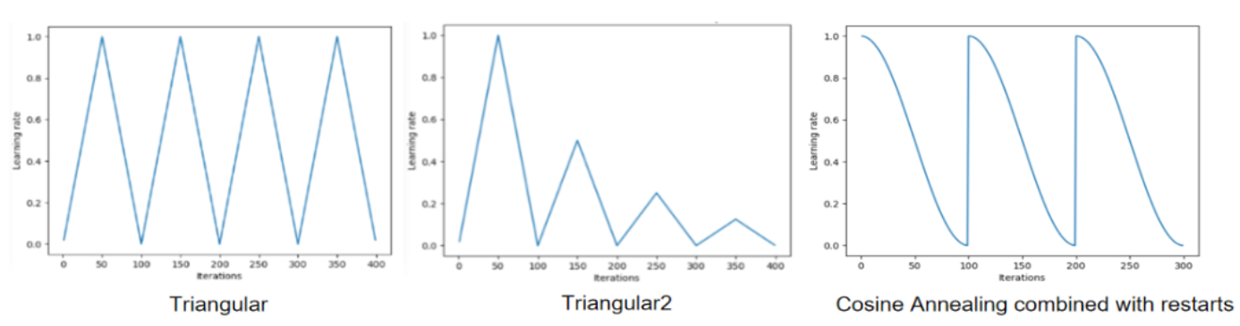
Cyclic Learning Rates
有多种形式,例如下图所示
二、正则化
L2(Weight Decay)
以二分类问题为例,使用L2正则化后的损失函数为:
$$\mathcal{J}=\underbrace{-\frac{1}{m} \sum\limits_{i = 1}^{m} [y^{(i)}\log\left(a^{[L] (i)}\right) + (1-y^{(i)})\log\left(1- a^{[L](i)}\right)]}_\text{cross-entropy cost} + \underbrace{\frac{\lambda}{2} \sum\limits_l\sum\limits_k\sum\limits_j W_{k,j}^{[l]2} }_\text{L2 regularization cost}$$
Dropout
网络的训练过程和文章神经网络介绍:算法基础中的基本一致,不同的是Dropout在每次迭代过程中随机关掉一些神经元,
对矩阵$A^{[l]}$,有对应的开关矩阵$D^{[l]}$,生成$D^{[l]}$的代码如下所示:
### 伪代码
Dl = np.random.rand(Al.shape[0], Al.shape[1])     # Step 1: initialize matrix D1 = np.random.rand(..., ...)
Dl = (Dl<keep_prob)                               # Step 2: convert entries of D1 to 0 or 1 (using keep_prob as the threshold)
(1)在前向传播过程中按上述文章中的公式计算出$A^{[l]}$后还需要额外进行处理:$$A^{[l]}=A^{[l]}*D^{[l]}\text{, }A^{[l]}=A^{[l]}/keep\_prob$$
(2)在后向传播过程中使用经过处理后的$A^{[l]}$进行计算,并且按文章中的公式计算出$dA^{[l]}$后还需要额外进行处理:$$dA^{[l]}=dA^{[l]}*D^{[l]}\text{, }dA^{[l]}=dA^{[l]}/keep\_prob$$
(3)需要注意的是在使用网络进行验证或预测时不要使用Dropout(即将keep_prob设为1)


 浙公网安备 33010602011771号