[REF]A quick guide teaching you how to use matlab to read netCDF file and plot a figure

1. Preparation. 4

2. A brief introduce to netCDF. 4

3. Data Structure. 4

3.1 Attributes. 7

3.2 Dimensions. 8

3.3 Variables. 9

Classfication. 10

3.4 Groups. 11

4. Source Code. 12

4.1 Get data from netCDF file. 12

4.2 Get subset data of specified variable. 13

Example 1: get the time series of a specified point (lon(11),lat(10))13

Example 2: get data of every point at time(0)14

4.3 Plot a figure 

1. Preparation

Software: Matlab 2014a;

Used netCDF File: example.nc(containd in Matlab Install files), pres.tropp.2015.nc.

Instruction/Reference:

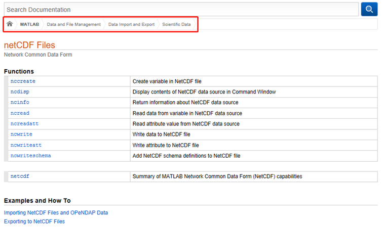
1. Matlab help documention

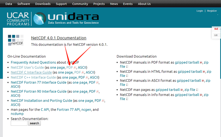
2. NetCDF User's Guide

https://www.unidata.ucar.edu/software/netcdf/old_docs/docs_4_0_1/

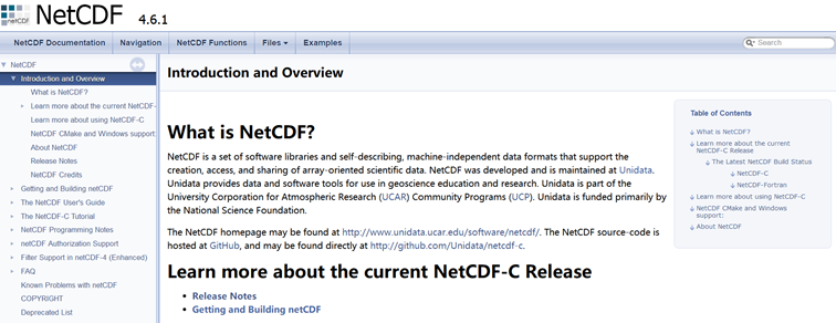
3. NetCDF Documentation

https://www.unidata.ucar.edu/software/netcdf/docs/index.html

2. A brief introduce to netCDF

NetCDF is a set of software libraries and self-describing, machine-independent data formats that support the creation, access, and sharing of array-oriented scientific data. NetCDF was developed and is maintained at Unidata. Unidata provides data and software tools for use in geoscience education and research.

Format	Model	Version	Released Year
Classic format	classic model	1.0~3.5	1989~2000
64-bit offset format		3.6	2004
netCDF-4 classic model format
	enhanced model (netCDF-4 data model)	4.0	2008
netCDF-4 format

l  data represented with the classic model can also be represented using the enhanced model;

l  datasets that use features of the enhanced model, such as user-defined nested data types, cannot be represented with the classic model;

l  Evolution will continue the commitment to keep the Backwards Compatibility;

n  Backwards means the “previous” and Forwards means the “future”;

l  Knowledge of format details is not required to read or write netCDF datasets, unless you want to understand the performance issues related to disk or server access.

l  The netCDF reference library, developed and supported by Unidata, is written in C,with Fortran77, Fortran90, and C++ interfaces. A number of community and commercially supported interfaces to other languages are also available, including IDL, Matlab, Perl,Python, and Ruby. An independent implementation, also developed and supported by Unidata, is written entirely in Java.

3. Data Structure

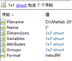
By use of the “ncinfo” we can get the structure information of the data source. This information is store in the Workspace. You can also use “ncdisp” to display the contents of the netCDF file in the Command Window.

structure1 = ncinfo('example.nc');	structure2 = ncinfo('pres.tropp.2015.nc')

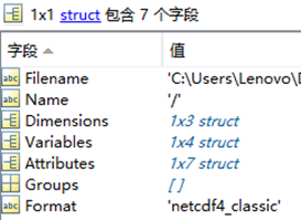 If we sort the data, we can get:

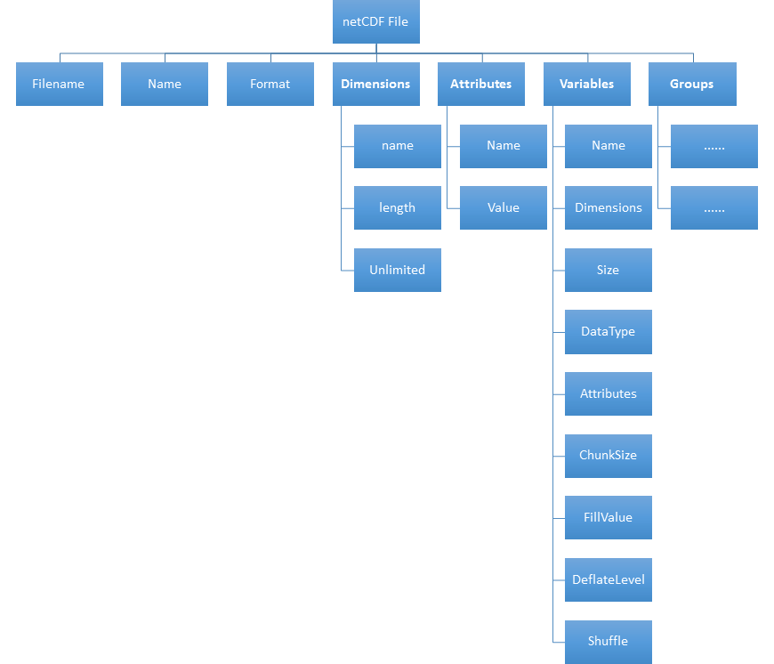
l  Filename: netCDF file name or URL.

l  Name: “/” indicating the full file

l  Format: the format of the netCDF file, see section 2.

l  Groups: An empty array([]) for all netCDF file format except netCDF-4 format.

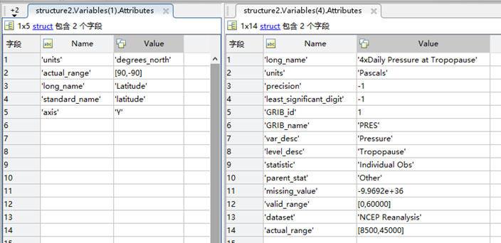
3.1 Attributes

概述：File有attributes，variable有attributes；就近原则，描述自己。

NetCDF attributes are used to store data about the data (ancillary data or metadata(元数据，描述数据的数据)), we can call them Global Attributes.

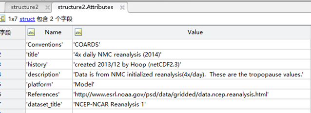
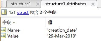
Most attributes provide information about a specific variable. These are identified by the name (or ID) of that variable, together with the name of the attribute.

 

 

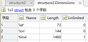
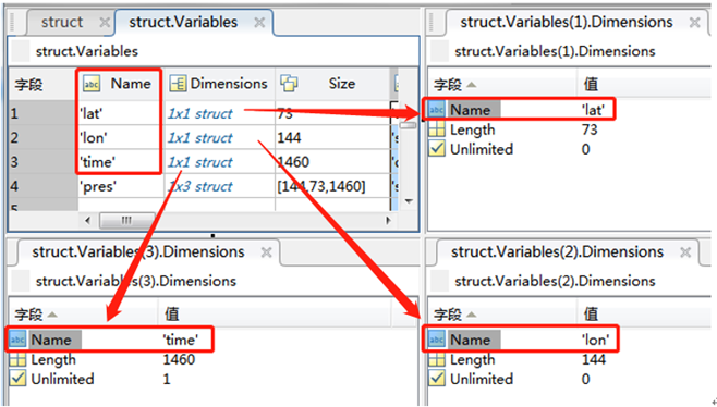
3.2 Dimensions

A dimension may be used to represent a real physical dimension, for example, time, latitude, longitude, or height. A dimension might also be used to index other quantities, for example station or People.

l  Name: the name of the dimension;

l  Length: number(sample) of values;

l  Unlimited: Boolean value. Indicates whether this dimension’s length is limited.

In a classic or 64-bit offset format dataset you can have at most one UNLIMITED dimension;

In a netCDF-4 format dataset, multiple UNLIMITED dimensions can be used.

3.3 Variables

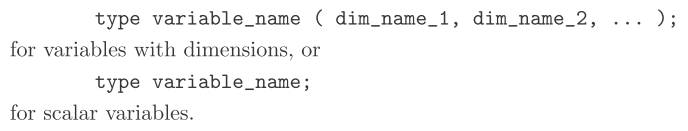
When a variable is defined, its shape is specified as a list of dimensions. These dimensions must already exist.

A scalar has no dimension, a vector has one dimension and a matrix has 2 dimensions.

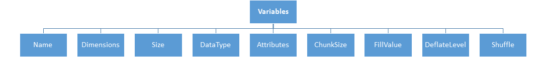
l  Dimensions: the same as “independent variables”.

l  Size: Like the matlab function “size” if the variable is matrix, like the matlab function “length” if the variable is verctor or scalar.

l  Attributes: see section 3.1

l  ChunkSize: specifying the size of one chunk. If the storage type specified is CONTIGUOUS it is “[]”.

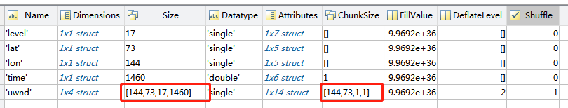
l  Fillvalue:Specifies the value to the variable when no other value is specified and use of fill values has been enabled.

最后这两个参数和数据的压缩有关，若数据是压缩过的，则需要解压后才能够读取。不过这些都是由底层的APIs(interface)实现的，我们可以不用管它。

l  DeflateLevel:Scalar value between 0 and 9 specifying the amount of compression, where 0 is no compression and 9 is the most compression

l  Shuffle:Boolean value. True indicates the shuffle filter is enabled for this variable. The shuffle filter can assist with the compression of integer data by changing the byte order in the data stream.

Classfication

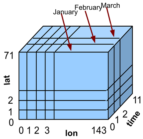
Class One: Coordinate variables

l  A variable with the same name as a dimension.

l  It typically defines a physical coordinate corresponding to that dimension.

n  So that you have alternative means of specifying position along the variable.

Index (C convention)	0	1	2	3	4	…
Index (Fortran convention)	1	2	3	4	5	…
physical coordinate (lat,lon,time etc.)	0	2.5	5	7.5	10	…

n  Matlab netCDF functions adopt C convention such that the counting starts from zero. Diagram below illustrates the actual index that we should use to extract the data using the Matlab functions.

 

http://www.public.asu.edu/~hhuang38/matlab_netcdf_guide.pdf

Class Two: Primary variables

l  This class can also be devied into two class:the Record variables and the others(just call it Fixed variables here)

l  Record variables: these variables has the unlimited dimension(like time), their size is variable.

l  Fixed variables: have a fixed size (number of data values) given by the product(叉乘、笛卡尔积) of its dimension lengths.

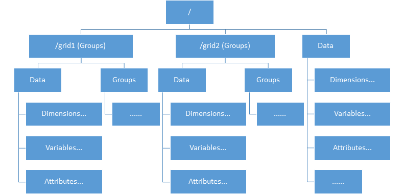
3.4 Groups

l  Starting with version 4.0, groups can help organize data within a dataset.

l  It’s not a type of data. Like a directory structure on a Unix file-system, the grouping feature allows users to organize variables and dimensions into distinct, named, hierarchical areas, called groups.

l  Here we use the file “example.nc” to demonstrate the groups’ structure

4. Source Code

After get know with the file structure, we can extract the data of specific “variables”. Here illustrate the step of process.

Step 0: use function “ncinfo” or “ncdisp” to check the structure and information of the netCDF file; (this step is unnecessary if you have got known with the data.)

Step 1: Open the file;

Step 2: Extract data from specific “variables”;

Step 3: close the file;

4.1 Get data from netCDF file

% get information/structure data

struct = ncinfo('pres.tropp.2015.nc');

% open the file(pres.tropp.2015.nc) by Read-only access(NC_NOWRITE)

% ncid is a NetCDF file identifier

ncid = netcdf.open('pres.tropp.2015.nc','NC_NOWRITE');

% get variable ID(varid) by given its name(pres)

varid = netcdf.inqVarID(ncid,'pres');

% get data(pres_data) by specifying the variable ID(varid)

pres_data = netcdf.getVar(ncid,varid);

% clos the file

netcdf.close(ncid);

% clear defunct parameters, leave alone the data(pres_data)

clear ncidvarid

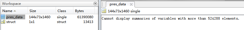
4.2 Get subset data of specified variable

The size of the “pres_data” matrix is 144×73×1460, what if I want to get the sub-matrix of “pres_data”?

Example 1: get the time series of a specified point (lon(11),lat(10))

ncid = netcdf.open('pres.tropp.2015.nc','NC_NOWRITE');

varid = netcdf.inqVarID(ncid,'pres');

series_data = netcdf.getVar(ncid,varid,[10,9,0],[1,1,1460]);

    % "[10,9,0]" represent the start point (Again, remember that counting starts from zero.)

    % "[1,1,1460]" specifies the amount of the data in each dimension.

% plot the data

% plot(series_data(:));

netcdf.close(ncid);

clear ncidvarid

• series_data is still a 3-dimention matrix, and the first two dimentions’ length is 1. The relation between “series_data” and “pres_data” is below:
• series_data(1,1,i) = pres_data(11,10,i),i=1,2,…,1460.

Example 2: get data of every point at time(0)

ncid = netcdf.open('pres.tropp.2015.nc','NC_NOWRITE');

varid = netcdf.inqVarID(ncid,'pres');

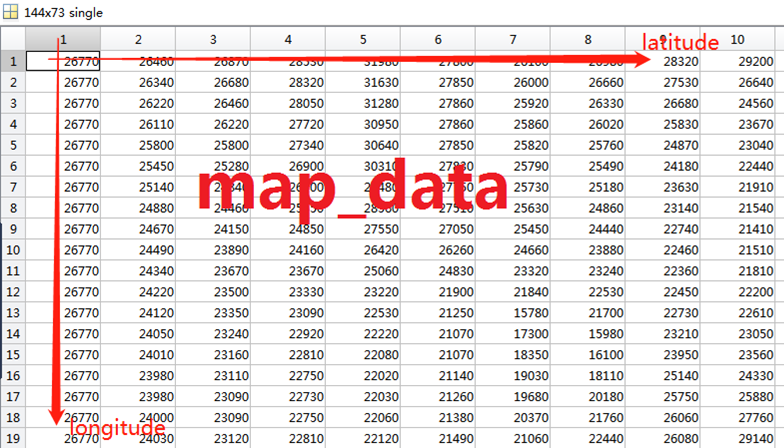
map_data = netcdf.getVar(ncid,varid,[0,0,0],[144,73,1]);

netcdf.close(ncid);

clear ncidvarid

• map_data is a 2-dimention matrix. The relation between “map_data” and “pres_data” is below:
• map_data(i,j) = pres_data(i,j,1),i=1,2,…,144;j=1,2,…,73

4.3 Plot a figure

% open the file

ncid = netcdf.open('pres.tropp.2015.nc','NC_NOWRITE');

% get data

map_data = netcdf.getVar(ncid,netcdf.inqVarID(ncid,'pres'),[0,0,0],[144,73,1]);

longitude = netcdf.getVar(ncid,netcdf.inqVarID(ncid,'lon'));

latitude = netcdf.getVar(ncid,netcdf.inqVarID(ncid,'lat'));

% Time = netcdf.getVar(ncid,netcdf.inqVarID(ncid,'time'));

% clos the file

netcdf.close(ncid);

% plot the data

map_data = map_data';  % map_data must be transposed(see below for details)

[x,y]=meshgrid(longitude,latitude);

pcolor(x,y,map_data); 

colorbar('location','eastoutside');

shading interp;colormap parula

% clear defunct parameters

clear ncidxy

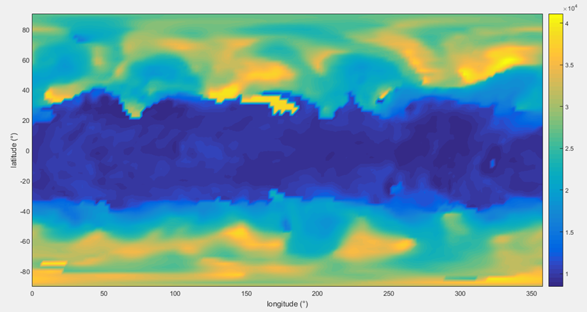
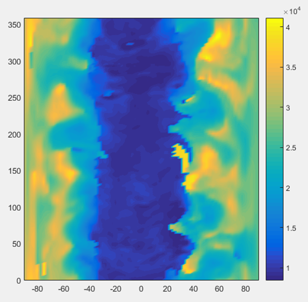
l  Be careful when you plot the figure, the 1^st dimension of the “map_data” is longitude, same as row of the matrix.

l  The y-axis of the figure will be “longitude” if “map_dat” is not transposed.