R语言5作图
生信技能树R语言部分学习笔记
1. 常用可视化R包
作图:base, ggplot2, ggpubr
拼图:par里的mfrow(基础包中图的拼接), grid.arrange, cowplot, customLayout, patchwork
导出:pdf()等三段论, ggsave(), eoffice----- topptx
2. 基础包——绘图函数
| 高级绘图函数 | 功能 | 低级绘图函数 | 功能 |
|---|---|---|---|
plot() |
绘制散点图等 | lines() |
添加线 |
hist() |
频率直方图 | curve() |
添加曲线 |
boxplot() |
箱线图 | abline() |
添加给定斜率的线 |
barplot() |
柱状图 | points() |
添加点 |
dotplot() |
点图 | segments() |
折线 |
piechart() |
饼图 | arrows() |
箭头 |
matplot() |
数学图形 | axis() |
坐标轴 |
stropchart() |
点图 | box() |
外框 |
title() |
标题 | ||
text() |
文字 | ||
mtext() |
图边文字 |
3. 基础包——绘图参数
参数用在函数内部,在没有设定值时使用默认值:
| 参数 | 含义 |
|---|---|
| font | 字体 |
| lty | 线类型 |
| lwd | 线宽度 |
| pch | 点的类型 |
| xlab | 横坐标 |
| ylab | 纵坐标 |
| xlim | 横坐标范围 |
| ylim | 纵坐标范围 |
也可以对整个要绘制图形的各种参数进行设定: par()
4. ggplot2语法
ggplot2的绘图主要分为以下几个方面:
- 入门级绘图模板
- 映射-颜色、大小、透明度、形状
- 分面
- 几何对象
- 统计变换
- 位置调整
- 坐标系
4.1 入门级模板
ggplot(data=<DATA>) + <GEOM_FUNCTION>(mapping=aes(<MAPPINGS>))
eg:
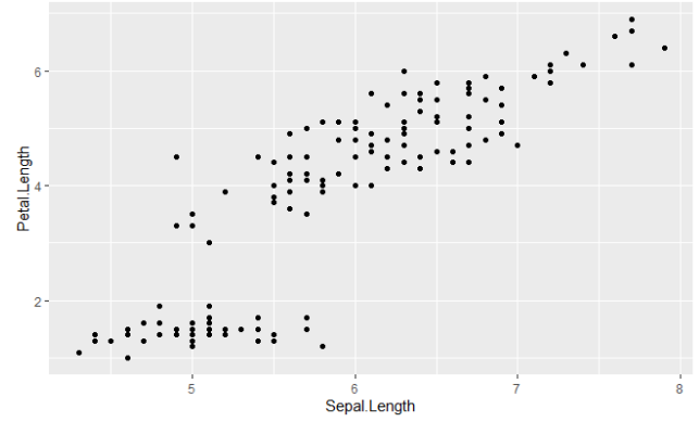
ggplot(data=iris)+
  geom_point(mapping=aes(x = Sepal.Length,
                         y = Petal.Length))
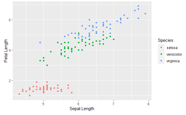
4.2 映射:按照数据框的某一列来定义图的某个属性
| 属性 | 参数 |
|---|---|
| x轴 | x |
| y轴 | y |
| 颜色 | color |
| 大小 | size |
| 形状 | shape |
| 透明度 | alpha |
| 填充颜色 | fill |
eg:
ggplot(data=iris)+
  geom_point(mapping=aes(x = Sepal.Length,
                         y = Petal.Length,
                         color = Species))
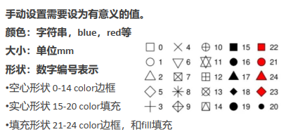
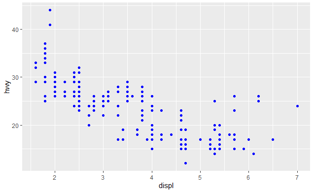
** 手动设置**
ggplot(data=mpg)+
  geom_point(mapping=aes(x = displ,
                         y = hwy),
                         color = "blue")
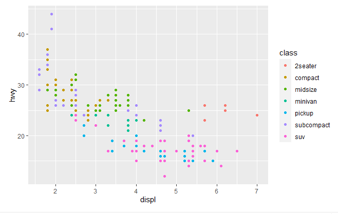
映射VS手动设置
映射的情况:是aes的参数,取值是列名
ggplot(data=mpg)+
  geom_point(mapping=aes(x = displ,
                         y = hwy,
                         color = class))
手动设置的情况:是geom_point的参数,取值是具体颜色
ggplot(data=mpg)+
  geom_point(mapping=aes(x = displ,
                         y = hwy),
                         color = "blue")
4.3 分面
(1) 单分面
ggplot(data = iris) +
  geom_point(mapping = aes(x = Sepal.Length, y = Petal.Length)) +
  facet_wrap(~ Species)
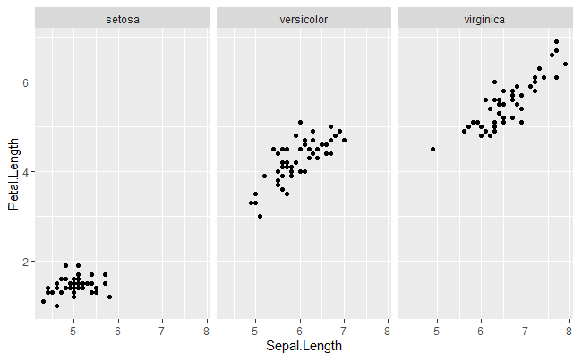
单分面的函数为facet_wrap(), 括号里面需要指定图片的列按照哪个变量划分,变量名写在波浪号右边。
(2) 双分面
test <- iris
test$group = sample(letters[1:5], 150, replace = T)

ggplot(data = test) +
  geom_point(mapping = aes(x = Sepal.Length, y = Petal.Length)) +
  facet_grid(group ~ Species)
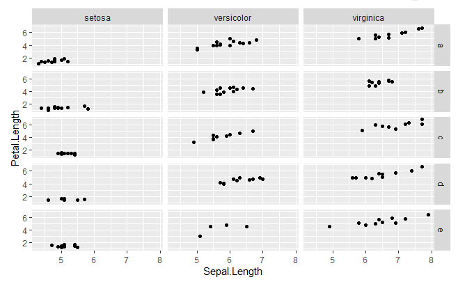
双分面的函数为facet_grid(), 括号里面需要指定图片的行和列按照哪个变量划分,波浪线左边对应于行划分,波浪线右边对应于列划分。
4.4 几何对象
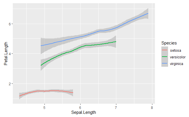
- 理解分组
ggplot(data = test) +
  geom_smooth(aes(x = Sepal.Length,
                  y = Petal.Length,
                  group = Species))
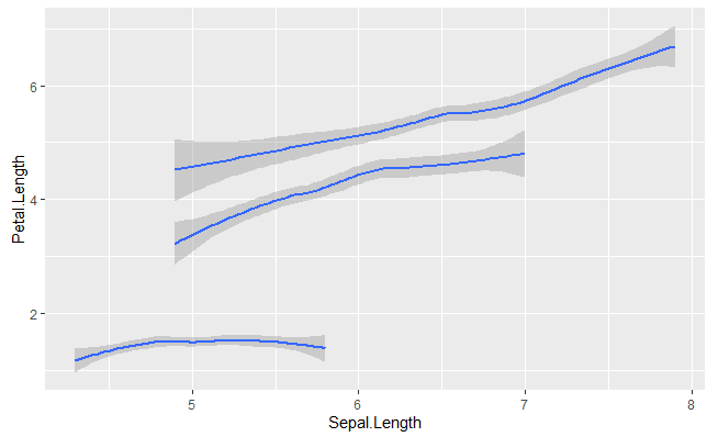
以下代码也可以达到分组的效果:
ggplot(data = test) +
  geom_smooth(aes(x = Sepal.Length,
                  y = Petal.Length,
                  color = Species))
- 几何对象可以叠加
ggplot(data = test) +
  geom_smooth(aes(x = Sepal.Length, y = Petal.Length)) +
  geom_point(aes(x = Sepal.Length, y = Petal.Length))

上面的代码等价于:
ggplot(data = test, mapping = aes(x = Sepal.Length, y = Petal.Length)) +
  geom_smooth() +
  geom_point()
放在geom_xxx()中的映射为局部映射,在ggplot()中的映射为全局映射。
映射分为局部映射和全局映射,局部映射仅对当前图层有效,全局映射对所有图层有效。
图层:geom_xxx()画出的单个集合对象。
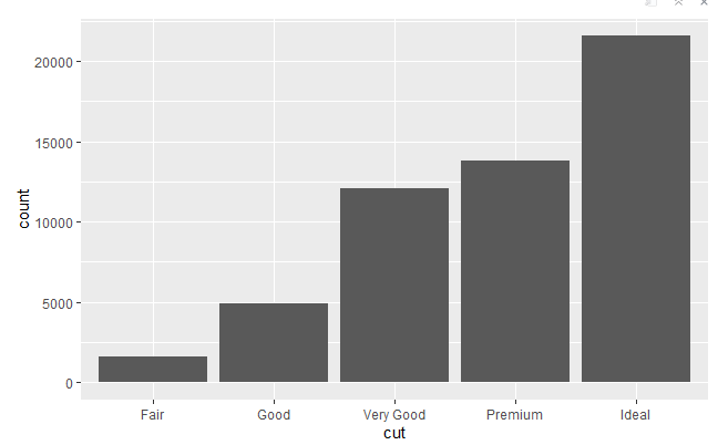
4.5 统计变换
直方图可以用函数geom_bar()生成,也可以用stat_count()生成。
ggplot(data = diamonds) +
  geom_bar(mapping = aes(x = cut))
和
ggplot(data = diamonds) +
  stat_count(mapping = aes(x = cut))
等价。
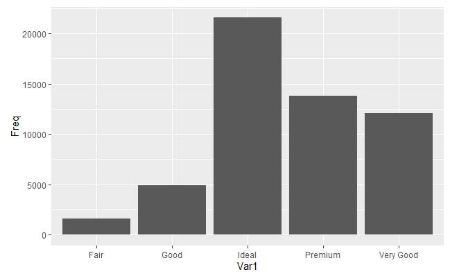
- 使用场景1:使用表中数据直接作图,而不统计

这里需要指定参数stat = "identity"
ggplot(data = fre) + geom_bar(mapping = aes(x = Var1, y = Freq),
                              stat = "identity")
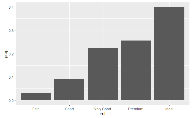
- 使用场景2:不统计count, 统计prop(比例)
ggplot(data = diamonds) +
  geom_bar(mapping = aes(x = cut, y = ..prop.., group = 1))
4.6 位置关系
当在箱线图上添加散点时,一般采用geom_jitter()代替geom_point(),防止出现点覆盖的情况。
堆叠直方图(主要体现比例)
ggplot(data = diamonds) +
  geom_bar(mapping = aes(x = cut,fill=clarity))
加上参数fill = clarity
并列直方图(主要体现大小关系)
ggplot(data = diamonds) +
  geom_bar(mapping = aes(x = cut, fill = clarity), position = "dodge")
加上position = "dodge"调整位置关系
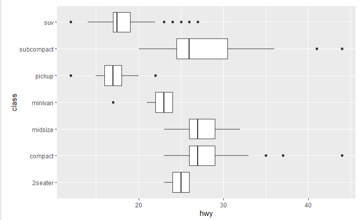
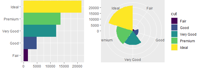
4.7 坐标系
coord_flip()翻转坐标系
ggplot(data = mpg, mapping = aes(x = class, y = hwy)) +
  geom_boxplot() +
  coord_flip()
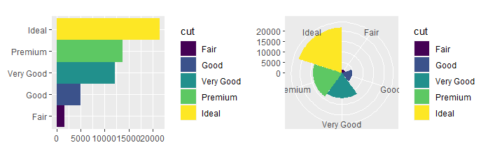
coord_polar()极坐标系
bar <- ggplot(data = diamonds) +
  geom_bar(
    mapping = aes(x = cut, fill = cut),
    show.legend = FALSE,
    width = 1
  ) +
  theme(aspect.ratio = 1) +
  labs(x = NULL, y = NULL)
bar
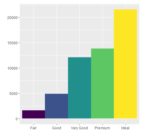
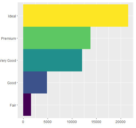
bar + coord_flip()
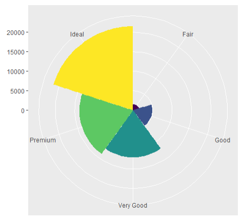
bar + coord_polar()
完整绘图模板

5. ggpubr
ggpubr是简化版ggplot
library(ggpubr)
ggscatter(iris,
          x="Sepal.Length",
          y="Petal.Length",
          color="Species")

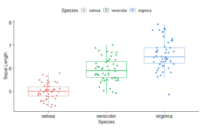
p <- ggboxplot(iris, x = "Species",
               y = "Sepal.Length",
               color = "Species",
               shape = "Species",
               add = "jitter")
p
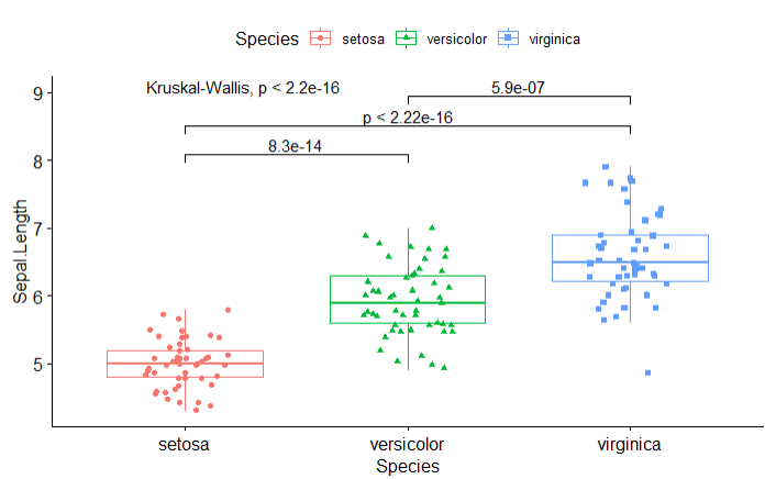
#添加组间比较
my_comparisons <- list( c("setosa", "versicolor"),
                        c("setosa", "virginica"),
                        c("versicolor", "virginica") )
p + stat_compare_means(comparisons = my_comparisons)+ # Add pairwise comparisons p-value
  stat_compare_means(label.y = 9)
6. 图片保存
- ggplot2系列
ggplot系列图(包括ggpubr)通用的简便保存ggsave
p <- ggboxplot(iris, x = "Species",
               y = "Sepal.Length",
               color = "Species",
               shape = "Species",
               add = "jitter")
ggsave(p,"iris_box_ggpubr.png")      #要求是画板上没有东西
- 通用:三段论
保存的格式及文件名-----> 作图代码 -----> 画完了,关闭画板
pdf("iris_box_ggpubr.pdf")
boxplot(iris[,1]~iris[,5])
text(6.5,4, labels = 'hello')
dev.off()
- 神器eoffice
导出为ppt,全部元素都是可编辑模式
library(eoffice)
topptx(p,"iris_box_ggpubr.pptx")
7. 拼图
R包patchwork
语法简单,完美兼容ggplot2
拼图比例设置简单
(1)支持直接p1 + p2拼图,比任何一个包都简单
#翻转coord_flip()
library(ggplot2)
ggplot(data = mpg, mapping = aes(x = class, y = hwy)) +
geom_boxplot() +
coord_flip()
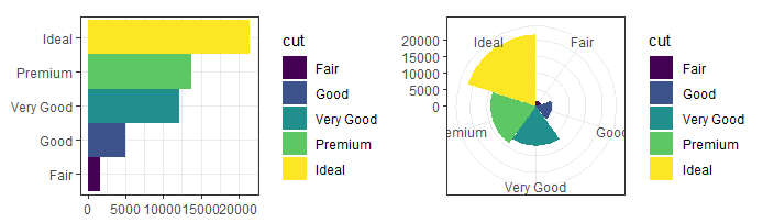
#极坐标系coord_polar()
bar <- ggplot(data = diamonds) +
geom_bar(
mapping = aes(x = cut, fill = cut),
#show.legend = FALSE,
width = 1
) +
theme(aspect.ratio = 1) +
labs(x = NULL, y = NULL)
bar + coord_flip()
bar + coord_polar()
p1 <- bar + coord_flip()
p2 <- bar + coord_polar()
#拼图
library(patchwork)
p1 + p2 #添加拼图 直接用 + 号
(2)复杂的布局代码易读性更强
(3)可以给子图添加标记(例如ABCD, I, II, III, IV)
p1 + p2 + plot_annotation(tag_levels = "A") #给图添加A,B,C,D编号

(4)可以统一修改所有子图
p1 + p2 & theme_bw() #整体去掉灰色背景
(5)可以将子图的图例收集到一起,整体性特别好
p1 + p2 + plot_layout(guides = "collect") #收集图例,只有patchwork包可以做
如何调整导出图片的比例?
dev.off()
ggsave(p2,filename = "p2.png",width = 10, height = 8)
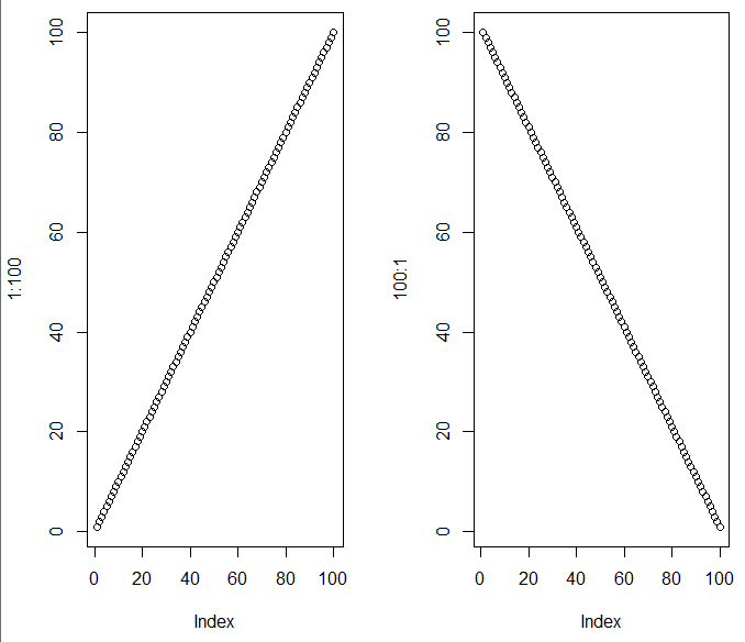
基础包拼图函数:
par(mfrow = c(2,2))
plot(1:100)
plot(100:1)
代码可运行却不出图可能是因为画板被占用
解决方案:多次运行dev.off(), 到null device为止,再运行出图代码
或dev.new()

 浙公网安备 33010602011771号