Matplotlib图例

 

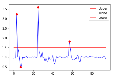
折线图示例

#!/usr/bin/python2.7

import numpy as np
from matplotlib import pyplot as plt
from dbtools import raw_data
from utils import moving_sum

def moving_sum(array, window):
    if type(array) is not np.ndarray:
        raise TypeError('Expected one dimensional numpy array.')

    remainder = array.size % window
    if 0 != remainder:
        array = array[remainder:]
    array = array.reshape((array.size/window,window))
    sum_arr = np.sum(array,axis=1)

    return sum_arr

def run():
    window = 3
    y_lst = raw_data('2018-08-03 00:00:00', length=3600*24)
    raw_arr = np.array(y_lst)

    sum_arr = moving_sum(raw_arr,window)
    res = np.true_divide(sum_arr[1:],sum_arr[:-1])
    
    threshold = 0.5
    upper = np.array([1+threshold]*res.size)
    lower = np.array([1-threshold]*res.size)
    
    plt.plot(upper,lw=1,color='red',label='Upper')
    plt.plot(res,lw=1,color='blue',label='Trend')
    plt.plot(lower,lw=1,color='red',label='Lower')

    r_idx = np.argwhere(np.abs(res-1) > 0.5)
    plt.plot(r_idx, res[r_idx], 'ro')

    plt.legend()
    plt.show()

    return (r_idx,res[r_idx])

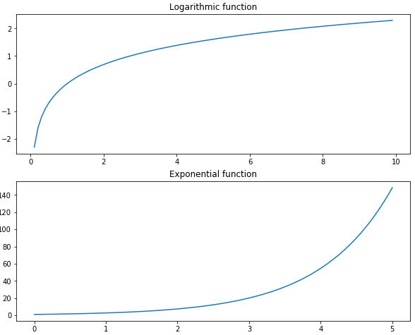
画布和子图

import numpy as np
import matplotlib.pyplot as plt

fig = plt.figure(figsize=[10,8])
ax1 = fig.add_subplot(2,1,1)
x1 = np.linspace(0.1,10,99,endpoint = False)
y1 = np.log(x1)
ax1.plot(x1,y1)
ax1.set_title('Logarithmic function')

x2 = np.linspace(0, 5, num = 100)
y2 = np.e**x2
ax2 = fig.add_subplot(2,1,2)
ax2.plot(x2,y2)
ax2.set_title('Exponential function')

plt.subplots_adjust(hspace =0.2)
fig.show()

 

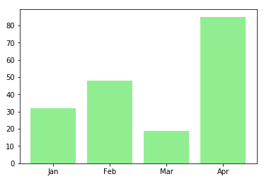
柱状图

import numpy as np
import matplotlib.pyplot as plt

data = [32,48,19,85]
labels = ['Jan','Feb','Mar','Apr']

plt.bar(np.arange(len(data)),data,color='lightgreen')
plt.xticks(np.arange(len(data)),labels)
plt.show()

 

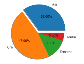
饼状图

import numpy as np
import matplotlib.pyplot as plt

data = [35,47,13,5]
labels = ['Bili','iQiYi','Tencent','YouKu']
plt.pie(data,labels=labels,autopct="%.2f%%",explode=[0.1,0,0,0],shadow=True)
plt.show()

 

Matplotlib画正弦余弦曲线 

 

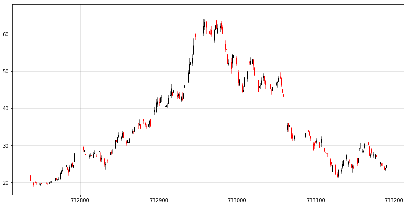
K线图

pip3.6 install https://github.com/matplotlib/mpl_finance/archive/master.zip

from mpl_finance import candlestick_ochl

# https://github.com/Gypsying/iPython/blob/master/601318.csv

In [2]: import pandas as pd                                                                                                                                                                                                               

In [3]: df = pd.read_csv('601318.csv', index_col='date', parse_dates=['date'])                                                                                                                                                            

In [4]: df.head()                                                                                                                                                                                                                         
Out[4]: 
            Unnamed: 0    open   close    high     low      volume    code
date                                                                      
2007-03-01           0  21.878  20.473  22.302  20.040  1977633.51  601318
2007-03-02           1  20.565  20.307  20.758  20.075   425048.32  601318
2007-03-05           2  20.119  19.419  20.202  19.047   419196.74  601318
2007-03-06           3  19.253  19.800  20.128  19.143   297727.88  601318
2007-03-07           4  19.817  20.338  20.522  19.651   287463.78  601318

In [5]: from matplotlib.dates import date2num                                                                                                                                                                                             

In [6]: df['time'] = date2num(df.index.to_pydatetime())                                                                                                                                                                                   

In [7]: df.head()                                                                                                                                                                                                                         
Out[7]: 
            Unnamed: 0    open   close    high     low      volume    code      time
date                                                                                
2007-03-01           0  21.878  20.473  22.302  20.040  1977633.51  601318  732736.0
2007-03-02           1  20.565  20.307  20.758  20.075   425048.32  601318  732737.0
2007-03-05           2  20.119  19.419  20.202  19.047   419196.74  601318  732740.0
2007-03-06           3  19.253  19.800  20.128  19.143   297727.88  601318  732741.0
2007-03-07           4  19.817  20.338  20.522  19.651   287463.78  601318  732742.0

In [8]: df.shape                                                                                                                                                                                                                          
Out[8]: (2563, 8)

In [9]: df.size                                                                                                                                                                                                                           
Out[9]: 20504

In [10]: 2563*8                                                                                                                                                                                                                           
Out[10]: 20504

In [11]: 

import numpy as np
import pandas as pd
from matplotlib.dates import date2num
from mpl_finance import candlestick_ochl

# 构建 candlestick_ochl 的sequence of (time, open, close, high, low, ...)
df = pd.read_csv('601318.csv', index_col='date', parse_dates=['date'])
# time must be in float days format - see date2num
df['time'] = date2num(df.index.to_pydatetime())
# 原始数据比较多，截取一部分做展示
df = df.iloc[:300,:]
arr = df[['time','open','close','high','low']].values

fig = plt.figure(figsize=[14,7])
ax = fig.add_subplot(1,1,1)

candlestick_ochl(ax,arr)

plt.grid(True, which='major', c='gray', ls='-', lw=1, alpha=0.2)
fig.show()