提取时序数据的趋势、季节性以及残差

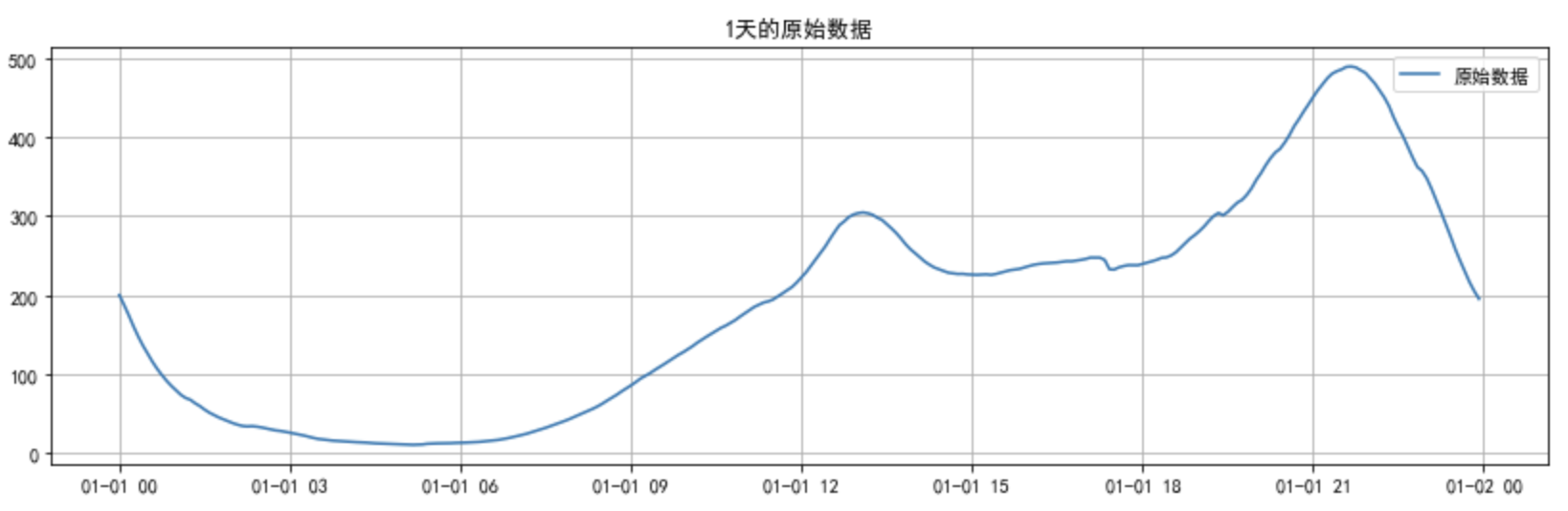
 一天的光滑数据

sub = [199.68, 187.16, 173.97, 159.85, 146.92, 135.29, 125.04, 114.86, 105.85, 97.93, 90.6, 84.19, 78.37, 72.85, 68.93, 66.59, 62.19, 58.59, 54.15, 50.26, 47.16, 44.14, 41.62, 38.99, 36.84, 34.9, 33.32, 32.75, 33.1, 32.49, 31.49, 30.13, 28.96, 27.72, 27.02, 26.01, 24.81, 23.64, 22.5, 21.14, 19.61, 18.08, 16.85, 16.08, 15.42, 14.71, 14.27, 13.85, 13.33, 12.85, 12.77, 12.5, 12.21, 11.68, 11.3, 11.07, 10.81, 10.57, 10.32, 9.99, 9.81, 9.59, 9.39, 9.54, 9.86, 10.72, 11.05, 11.2, 11.28, 11.41, 11.51, 11.84, 11.87, 12.17, 12.44, 12.75, 13.09, 13.69, 14.32, 14.98, 15.62, 16.62, 17.78, 19.08, 20.53, 22.03, 23.48, 25.33, 26.91, 28.88, 31.03, 33.17, 35.28, 37.6, 39.7, 42.09, 44.84, 47.6, 50.08, 52.63, 55.35, 58.39, 61.85, 65.73, 69.26, 73.01, 77.22, 80.93, 84.9, 89.03, 93.53, 97.01, 100.34, 104.42, 108.11, 111.9, 115.88, 119.73, 123.65, 127.0, 130.81, 134.72, 139.23, 143.22, 146.97, 150.6, 154.12, 158.0, 160.79, 164.26, 167.85, 172.3, 176.39, 180.55, 184.54, 187.43, 190.19, 191.72, 194.04, 197.86, 201.93, 205.85, 209.98, 215.71, 222.41, 228.96, 237.09, 245.32, 252.96, 261.38, 271.01, 280.07, 288.58, 293.28, 298.88, 302.11, 303.89, 304.67, 303.63, 301.74, 297.96, 295.17, 289.9, 284.35, 278.44, 271.56, 264.14, 257.84, 252.81, 247.4, 242.34, 238.34, 234.8, 232.4, 230.27, 228.12, 227.27, 226.53, 226.7, 225.94, 225.77, 225.4, 225.77, 226.03, 225.37, 226.46, 228.19, 229.69, 231.28, 232.03, 232.97, 234.78, 236.51, 238.08, 239.13, 239.85, 240.21, 240.7, 241.1, 241.95, 242.71, 242.62, 243.52, 244.39, 245.62, 247.28, 247.29, 247.2, 244.31, 232.43, 232.11, 234.95, 236.59, 237.73, 237.79, 237.62, 239.26, 240.68, 242.67, 244.52, 246.94, 247.55, 249.97, 253.92, 259.84, 265.83, 271.51, 275.89, 281.14, 287.01, 293.99, 300.1, 304.04, 301.13, 305.42, 311.59, 317.24, 320.75, 327.11, 335.54, 346.18, 354.8, 364.94, 373.74, 380.87, 385.53, 393.56, 403.18, 414.45, 423.33, 433.06, 441.96, 451.35, 460.2, 467.68, 475.33, 481.09, 484.22, 486.48, 489.69, 490.18, 489.02, 485.48, 482.26, 475.31, 468.71, 460.07, 451.05, 440.02, 425.39, 412.68, 401.18, 388.03, 374.44, 362.4, 357.28, 347.81, 334.59, 320.07, 304.97, 289.75, 274.3, 258.01, 243.51, 229.82, 216.16, 204.78, 194.9]
index = pd.date_range('2018-01-01', periods=288, freq='5T')  # 从某个日期开始，每 5 分钟一个数据点
ts = pd.Series(sub, index=index)
plt.figure(figsize=(14, 4))
plt.plot(ts, label='原始数据')
plt.title("1天的原始数据", fontproperties=zhfont, fontsize=12)
plt.grid()
plt.legend()

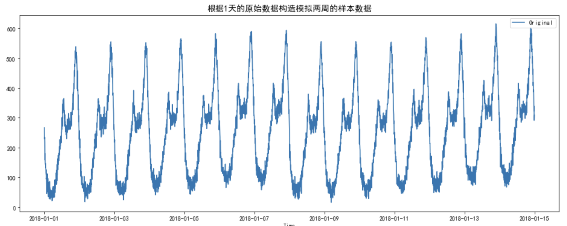
基于一天的数据构造两周的毛刺数据

import numpy as np
import pandas as pd
import matplotlib.pyplot as plt
from matplotlib import font_manager
fname="/usr/local/python3.6/lib/python3.6/site-packages/matplotlib/mpl-data/fonts/ttf/simhei.ttf"
zhfont = font_manager.FontProperties(fname=fname)
from statsmodels.tsa.seasonal import seasonal_decompose

# 设置随机种子以便结果可复现
np.random.seed(0)

# 将每日数据扩展至14天
one_day_data = sub
one_day_data = np.array(one_day_data)
n_days = 14  # 14 days of data (two weeks)
n_points = n_days * len(one_day_data)  # 总共的数据点数
daily_data = np.tile(one_day_data, n_days)

# 构造长期趋势：保持稳定并有小幅度上涨的平滑趋势
trend = 0.001 * np.arange(n_points)  # 使用一个较小的线性增长趋势
# 每周季节性成分：周期为7天，每周重复，周末人数增多
weekly_pattern = np.array([39, 46, 48, 60, 61, 87, 85])  # 周一到周日的用户波动模式
seasonal_weekly = np.tile(np.repeat(weekly_pattern, len(one_day_data)), n_days // 7 + 1)[:n_points]  # 匹配至完整数据点数
# 随机噪声
noise = np.random.normal(0, 16, n_points)  # 降低噪声幅度以保持数据更平滑
# 合成信号 = 趋势 + 每周季节性 + 每日季节性 + 噪声
signal = trend + seasonal_weekly + daily_data + noise


# 将数据放入 pandas Series
index = pd.date_range('2018-01-01', periods=n_points, freq='5T')  # 从某个日期开始，每 5 分钟一个数据点
ts = pd.Series(signal, index=index)


# 绘制构造结果
plt.figure(figsize=(16, 6))
plt.plot(ts, label='Original')
plt.title('根据1天的原始数据构造模拟两周的样本数据', fontproperties=zhfont, fontsize=14)
plt.xlabel('Time')
plt.legend(loc='best')
# plt.grid()
plt.show()

 

 方法一：使用statsmodels提取

import numpy as np
import pandas as pd
import matplotlib.pyplot as plt
from matplotlib import font_manager
fname="/usr/local/python3.6/lib/python3.6/site-packages/matplotlib/mpl-data/fonts/ttf/simhei.ttf"
zhfont = font_manager.FontProperties(fname=fname)
from statsmodels.tsa.seasonal import seasonal_decompose


# 使用 statsmodels 进行季节性分解
# 设定每周的周期
result_weekly = seasonal_decompose(ts, period=len(one_day_data) * 7, model='additive')
# 获取分解结果
trend_component = result_weekly.trend
seasonal_component = result_weekly.seasonal
residual_component = result_weekly.resid


# 绘制分解结果
plt.figure(figsize=(12, 9))
plt.subplot(3, 1, 1)
plt.plot(trend_component, label='Trend')
plt.title('长期趋势', fontproperties=zhfont, fontsize=12)
plt.xlabel('Time')
plt.legend(loc='best')

plt.subplot(3, 1, 2)
plt.plot(seasonal_component, label='Seasonal (Weekly)')
plt.title('每周季节性')
plt.xlabel('Time')
plt.legend(loc='best')

plt.subplot(3, 1, 3)
plt.plot(residual_component, label='Residual')
plt.title('残差')
plt.xlabel('Time')
plt.legend(loc='best')

plt.tight_layout()
plt.show()