RANS的涡流粘度模型

The Reynolds-averaged Navier-Stokes(RANS) equations are:

\[\frac{\partial\left(\rho U_i\right)}{\partial t}+\frac{\partial}{\partial x_j}\left(\rho U_iU_j\right)=-\frac{\partial P}{\partial x_i}+\frac{\partial}{\partial x_j}\left[\mu\left(\frac{\partial U_i}{\partial x_j}+\frac{\partial U_j}{\partial x_i}\right)-\rho\overline{\boldsymbol{u'}_i\boldsymbol{u'}_j}\right] \]

The Reynolds-averaging process results in an additional stress term:

\[-\rho\overline{\boldsymbol{u'}_i\boldsymbol{u'}_j} \]

In order to solve the RANS equations, we need to express the Reynolds Stress interms of the mean flow quantities.
This is the turbulence closure problem.

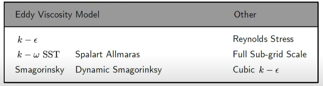
Eddy Viscosity Models(涡流粘度模型)

Eddy viscosity models are a class of turbulence model that are used to calculate the Reynolds stresses(\(-\rho\overline{\boldsymbol{u'}_i\boldsymbol{u'}_j}\))

How do Eddy Viscosity Models work?

Shear Flow

Consider a simple shear flow in 2D

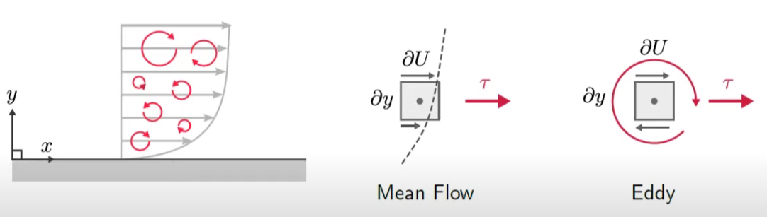
The fluid element is sheared by the mean flow and by the eddy

The shear stress from the mean flow(viscous shear) is:

\[\tau=\mu\frac{\partial U}{\partial y}\quad(3) \]

The shear stress from the eddies / turbulence is given by the Reynolds stress:
(涡流/湍流产生的剪切应力由雷诺应力给出：)

\[\tau=-\rho\overline{u'v'}\quad(4) \]

In RANS, we don't calculate the fluctuating velocity components \(u'\)and \(v'\) directly.
We model them by somehow relating them to the mean flow variables (U, V, W).

Brownian Motion

Assume that turbulent fluctuations are analogous to Brownian motion of gas particles.(假设湍流波动类似于气体粒子的布朗运动。)

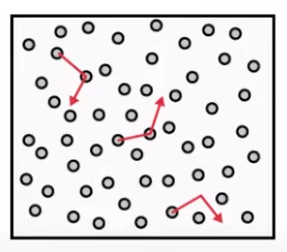
In Brownian motion, particles collide with each other, exchanging energy and momentum.
The motion of individual particles is random.

The Brownian particles are also moved by the background fluid motion.
In a sheared flow, the lower particles are accelerated by the faster moving fluid above them.

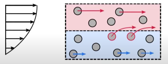
Particles accelerated by fast fluid above(粒子被上面的快速流体加速)

There is a net transport of momentum to the lower particles (downwards)
(动量净传输到较低的粒子（向下）)

Eddy Viscosity Models

In the previous example, the momentum is transported downwards.
In general, momentum is transported in the direction of the velocity gradient.
Therefore, assume that the Reynolds stress is proportional to \(\partial U/\partial y\)
(一般来说，动量沿速度梯度方向传递，因此，假设雷诺应力与\(\partial U/\partial y\)成正比)

\[-\rho\overline{u'v'}=\mu_t\frac{\partial U}{\partial y}\quad(5) \]

The constant of proportionality is called the eddy / turbulent viscosity \(\mu_t\).
\(\mu_t\) is artificial and controls the strength of diffusion. Further modelling is needed to calculate \(\mu_t\).

Brownian Motion

If the turbulent fluctuations are stronger, the Brownian motion is stronger
We expect the lower particles to be accelerated more by the collisions

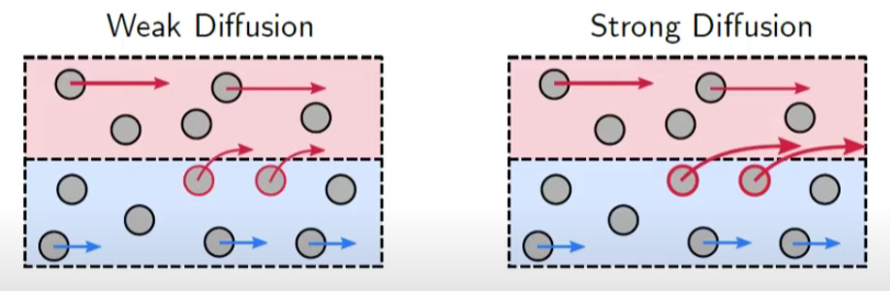
The diffusion is always in the same direction (the mean velocity gradient)
\(\mu_t\) controls the strength of the diffusion (strength of the collisions)

Nomenclature(命名法)

\[-\rho\overline{u^{\prime}v^{\prime}}=\mu_{t}\frac{\partial U}{\partial y}\quad(6) \]

This assumption was first introduced by Boussinesq in 1877.
Hence, it is sometimes called the Boussinesq approximation, Boussinesq hypothesis and sometimes an eddy viscosity model.
(它有时被称为 Boussinesq 近似、Boussinesq 假设，有时被称为涡粘模型)
How can we extend this model to 3D?

Eddy Viscosity Models in 3D

From the analysis of the simple shear flow we have:

\[-\rho\overline{u^{\prime}v^{\prime}}=\mu_{t}\frac{\partial U}{\partial y}\quad(7) \]

Write the same equation for a shear profile in the y direction

\[-\rho\overline{v^{\prime}u^{\prime}}=\mu_{t}\frac{\partial V}{\partial x}\quad(8) \]

But the order of multiplication does not matter(\(-\rho\overline{u^{\prime}v^{\prime}}=-\rho\overline{v^{\prime}u^{\prime}}\))

Therefore:

\[-\rho\overline{u'v'}=\mu_t\left(\frac{\partial U}{\partial y}+\frac{\partial V}{\partial x}\right)\quad(9) \]

Now we are going to consider the normal components (\(u'u'\)). Let \(v'=u'\)

\[\begin{aligned}-\rho\overline{u'u'}&=\mu_t\left(\frac{\partial U}{\partial x}+\frac{\partial U}{\partial x}\right)&(11)\\-\rho\overline{u'u'}&=2\mu_t\frac{\partial U}{\partial x}&(12)\end{aligned} \]

There is a small problem here...
The definition of turbulent kinetic energy tells us:

\[k=\frac12\left(\overline{u'u'}+\overline{v'v'}+\overline{w'w'}\right)\quad(13) \]

Hence, the sum of the normal turbulent stresses should give:
(因此，法向湍流应力的总和应为：)

\[\begin{aligned} -(\rho\overline{u^{\prime}u^{\prime}}+\rho\overline{v^{\prime}v^{\prime}}+\rho\overline{w^{\prime}w^{\prime}})& =-\rho(\overline{u^{\prime}u^{\prime}}+\overline{v^{\prime}v^{\prime}}+\overline{w^{\prime}w^{\prime}}) \\ &=-2\rho k \end{aligned}\]

But if we add our three normal stresses together we get:

\[-(\rho\overline{u'u'}+\rho\overline{v'v'}+\rho\overline{w'w'})=2\mu_{t}\left(\frac{\partial U}{\partial x}+\frac{\partial V}{\partial y}+\frac{\partial W}{\partial z}\right)\quad(16) \]

If the flow is incompressible then the continuity equation tells us that:

\[\begin{aligned}\frac{\partial U}{\partial x}+\frac{\partial V}{\partial y}+\frac{\partial W}{\partial z}&=0\quad(18)\end{aligned} \]

Hence:

\[-(\rho\overline{u'u'}+\rho\overline{v'v'}+\rho\overline{w'w'})=0\quad[\text{Incompressible Flows}]\quad\quad(19) \]

This is clearly incorrect.(这显然是不正确的。)

\[-(\rho\overline{u'u'}+\rho\overline{v'v'}+\rho\overline{w'w'})\neq2\mu_t\left(\frac{\partial U}{\partial x}+\frac{\partial V}{\partial y}+\frac{\partial W}{\partial z}\right)\quad(20) \]

What do we do to correct the calculation of the normal stresses?
Subtract 1/3rd of the error from each of the normal components.
我们如何修正法向应力的计算？
从每个正常分量中减去 1/3 的误差。

\[\begin{gathered} -\rho\overline{u^{\prime}u^{\prime}} =2\mu_{t}\left(\frac{\partial U}{\partial x}-\frac{1}{3}\left(\frac{\partial U}{\partial x}+\frac{\partial V}{\partial y}+\frac{\partial W}{\partial z}\right)\right)-\frac{1}{3}\left(2\rho k\right) \quad\left({21}\right) \\ -\rho\overline{v^{\prime}v^{\prime}} =2\mu_{t}\left(\frac{\partial V}{\partial y}-\frac13\left(\frac{\partial U}{\partial x}+\frac{\partial V}{\partial y}+\frac{\partial W}{\partial z}\right)\right)-\frac13\left(2\rho k\right) \quad(22) \\ -\rho\overline{w^{\prime}w^{\prime}} =2\mu_{t}\left(\frac{\partial W}{\partial z}-\frac{1}{3}\left(\frac{\partial U}{\partial x}+\frac{\partial V}{\partial y}+\frac{\partial W}{\partial z}\right)\right)-\frac{1}{3}\left(2\rho k\right) \quad(23) \end{gathered}\]

As a check, add the normal stresses together and we got the turbulent kinetic energy!

\[\begin{aligned} -(\rho\overline{u'u'}+\rho\overline{v'v'}+\rho\overline{w'w'})=2\mu_{t}\left(\frac{\partial U}{\partial x}+\frac{\partial V}{\partial y}+\frac{\partial W}{\partial z}-\right. \\ \left.\left(\frac{\partial U}{\partial x}+\frac{\partial V}{\partial y}+\frac{\partial W}{\partial z}\right)\right)-2\rho k& \quad(24) \\ -(\rho\overline{u'u'}+\rho\overline{v'v'}+\rho\overline{w'w'})=-2\rho k& \quad(25) \\ {k=\frac{1}{2}\left(\overline{u'u'}+\overline{v'v'}+\overline{w'w'}\right)}& \quad(26) \end{aligned}\]

Summary

For the shear stresses we calculated:

\[-\rho\overline{u'v'}=\mu_t\left(\frac{\partial U}{\partial y}+\frac{\partial V}{\partial x}\right)\quad(27) \]

And for the normal stresses we calculated:

\[-\rho\overline{u'u'}=2\mu_t\left(\frac{\partial U}{\partial x}-\frac{1}{3}\left(\frac{\partial U}{\partial x}+\frac{\partial V}{\partial y}+\frac{\partial W}{\partial z}\right)\right)-\frac{1}{3}\left(2\rho k\right)\quad(28) \]

We would like to write this in a more compact form that is valid for both normal and shear components

Introducing Tensor(i,j) Notation

Introducing Tensor(i,j) Notation, we can write the shear stresses as:

\[-\rho\overline{u_i'u'_j}=\mu_t\left(\frac{\partial U_i}{\partial x_j}+\frac{\partial U_j}{\partial x_i}\right)\quad(29) \]

And we can write the normal stresses as:

\[-\rho\overline{u'_iu'_j}=\mu_t\left(\frac{\partial U_i}{\partial x_j}+\frac{\partial U_j}{\partial x_i}-\frac{2}{3}\frac{\partial U_k}{\partial x_k}\right)-\frac{2}{3}\rho k\quad(30) \]

The repeated indices (k,k) indicate summation / contraction.
How can we combine the normal and shear stresses into one formula?
(重复的索引(k,k)表示求和/收缩。我们如何将法向应力和剪应力合并到一个公式中？)

Kronecker Delta

We can combine the normal and shear stress equations together using the Kronecker Delta symbol \(\delta_{ij}\)

\[\delta_{ij}=\begin{cases}1&\quad i=j\\0&\quad i\neq j\end{cases}\quad(31) \]

Multiply the extra terms in the normal components by the Kronecker delta.
They will vanish when i≠,j! Hence we can bring everything together:
(将正常分量中的额外项乘以克罗内克增量。当 i≠,j 时它们就会消失！ 因此我们可以将所有内容整合在一起：)

\[-\rho\overline{u_{i}^{\prime}u_{j}^{\prime}}=\mu_{t}\left(\frac{\partial U_{i}}{\partial x_{j}}+\frac{\partial U_{j}}{\partial x_{i}}-\frac{2}{3}\frac{\partial U_{k}}{\partial x_{k}}\delta_{ij}\right)-\frac{2}{3}\rho k\delta_{ij}\quad(32) \]

This equation is valid for both the shear and normal components!

We can also write this equation in vector form.

\[-\rho\overline{\boldsymbol{u'u'}}=\mu_{t}\left((\nabla\boldsymbol{U})+(\nabla\boldsymbol{U})^{T}-\frac{2}{3}\left(\nabla\cdot\boldsymbol{U}\right)\boldsymbol{I}\right)-\frac{2}{3}\rho k\boldsymbol{I}\quad(34) \]

Use whichever version you prefer.
Notice that the kronecker delta \(\delta_{ij}\) is equal to the identity matrix \(I\)!

\[\delta_{ij}=\begin{cases}1&\quad i=j\\0&\quad i\neq j\end{cases}\quad=\begin{bmatrix}1&0&0\\0&1&0\\0&0&1\end{bmatrix}\quad(35) \]

Concise Form(简洁形式)

\[-\rho\overline{u_{i}^{\prime}u_{j}^{\prime}}=\mu_{t}\left(\frac{\partial U_{i}}{\partial x_{j}}+\frac{\partial U_{j}}{\partial x_{i}}-\frac{2}{3}\frac{\partial U_{k}}{\partial x_{k}}\delta_{ij}\right)-\frac{2}{3}\rho k\delta_{ij}\quad(36) \]

This form of the equation is quite long.
Can we write it in a more compact way?

Strain Rate Tensor(应变率张量)

We can use the mean rate of strain tensor \(S_{i,j}\), which is defined as:

\[\begin{aligned}S_{ij}&=\frac{1}{2}\left(\frac{\partial U_i}{\partial x_j}+\frac{\partial U_j}{\partial x_i}\right)\quad(37)\end{aligned} \]

Or even more compact, we can use the deviatoric part of this tensor \(S_{ij}^{\star}\)

\[S_{ij}^{\star}=\frac{1}{2}\left(\frac{\partial U_{i}}{\partial x_{j}}+\frac{\partial U_{j}}{\partial x_{i}}-\frac{1}{3}\frac{\partial U_{k}}{\partial x_{k}}\delta_{ij}\right)\quad(38) \]

Many authors use the deviatoric part to make the equation compact. lt has no
special meaning.

Concise Form

\[\begin{aligned} -\rho\overline{u_{i}^{\prime}u_{j}^{\prime}}& =2\mu_{t}\left(S_{ij}-\frac{1}{3}\frac{\partial U_{k}}{\partial x_{k}}\delta_{ij}\right)-\frac{2}{3}\rho k\delta_{ij} && \text{(39)} \\ &-\rho\overline{u_{i}^{\prime}u_{j}^{\prime}}=2\mu_{t}S_{ij}^{\star}-\frac{2}{3}\rho k\delta_{ij}&& \left.\left(\begin{matrix}{40}\\\end{matrix}\right.\right) \end{aligned}\]

How is \(\mu_t\) calculated?

\(\mu_t\) is calculated with the chosen turbulence model (like \(k-\epsilon\))
We solve an equation for k and \(\epsilon\) , which allows us to calculate \(\mu_t\)

\[\mu_t=\rho C_\mu\frac{k^2}{\epsilon}\quad[k-\epsilon]\quad(41) \]

Once \(\mu_t\) has been calculated, use the eddy viscosity hypothesis to calculate the Reynolds stresses.