Self-Taught Learning to Deep Networks

 

In this section, we describe how you can fine-tune and further improve the learned features using labeled data. When you have a large amount of labeled training data, this can significantly improve your classifier's performance.

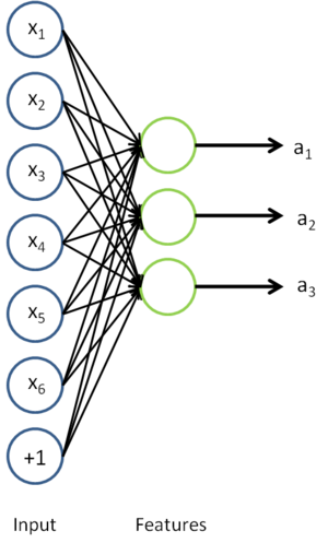
In self-taught learning, we first trained a sparse autoencoder on the unlabeled data. Then, given a new example , we used the hidden layer to extract features . This is illustrated in the following diagram:

 

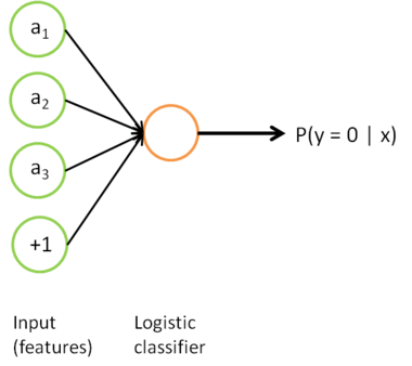
We are interested in solving a classification task, where our goal is to predict labels . We have a labeled training set of labeled examples. We showed previously that we can replace the original features with features computed by the sparse autoencoder (the "replacement" representation). This gives us a training set . Finally, we train a logistic classifier to map from the features to the classification label .

we can draw our logistic regression unit (shown in orange) as follows:

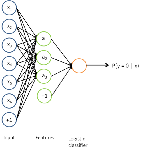
Now, consider the overall classifier (i.e., the input-output mapping) that we have learned using this method. In particular, let us examine the function that our classifier uses to map from from a new test example to a new prediction p(y = 1 | x). We can draw a representation of this function by putting together the two pictures from above. In particular, the final classifier looks like this:

The parameters of this model were trained in two stages: The first layer of weights mapping from the input to the hidden unit activations were trained as part of the sparse autoencoder training process. The second layer of weights mapping from the activations to the output was trained using logistic regression (or softmax regression).

But the form of our overall/final classifier is clearly just a whole big neural network. So, having trained up an initial set of parameters for our model (training the first layer using an autoencoder, and the second layer via logistic/softmax regression), we can further modify all the parameters in our model to try to further reduce the training error. In particular, we can fine-tune the parameters, meaning perform gradient descent (or use L-BFGS) from the current setting of the parameters to try to reduce the training error on our labeled training set .

When fine-tuning is used, sometimes the original unsupervised feature learning steps (i.e., training the autoencoder and the logistic classifier) are called pre-training. The effect of fine-tuning is that the labeled data can be used to modify the weights W⁽¹⁾ as well, so that adjustments can be made to the features a extracted by the layer of hidden units.

if we are using fine-tuning usually we will do so with a network built using the replacement representation. (If you are not using fine-tuning however, then sometimes the concatenation representation can give much better performance.)

When should we use fine-tuning? It is typically used only if you have a large labeled training set; in this setting, fine-tuning can significantly improve the performance of your classifier. However, if you have a large unlabeled dataset (for unsupervised feature learning/pre-training) and only a relatively small labeled training set, then fine-tuning is significantly less likely to help.