Exercise : Softmax Regression
Step 0: Initialize constants and parameters
Step 1: Load data
Step 2: Implement softmaxCost
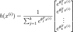
Implementation Tip: Preventing overflows - in softmax regression, you will have to compute the hypothesis
When the products
are large, the exponential function
will become very large and possibly overflow. When this happens, you will not be able to compute your hypothesis. However, there is an easy solution - observe that we can multiply the top and bottom of the hypothesis by some constant without changing the output:
Hence, to prevent overflow, simply subtract some large constant value from each of the
terms before computing the exponential. In practice, for each example, you can use the maximum of the
terms as the constant. Assuming you have a matrix M containing these terms such that M(r, c) is
, then you can use the following code to accomplish this:
% M is the matrix as described in the text
M = bsxfun(@minus, M, max(M, [], 1));
Implementation Tip: Computing the predictions - you may also find bsxfun useful in computing your predictions - if you have a matrix M containing the
terms, such that M(r, c) contains the
term, you can use the following code to compute the hypothesis (by dividing all elements in each column by their column sum):
% M is the matrix as described in the text
M = bsxfun(@rdivide, M, sum(M))
 are large, the exponential function
  will become very large and possibly overflow. When this happens, you will not be able to compute your hypothesis. However, there is an easy solution - observe that we can multiply the top and bottom of the hypothesis by some constant without changing the output:
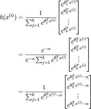
 terms before computing the exponential. In practice, for each example, you can use the maximum of the
  , then you can use the following code to accomplish this:
 terms, such that M(r, c) contains the
  term, you can use the following code to compute the hypothesis (by dividing all elements in each column by their column sum):
Step 3: Gradient checking
Implementation Tip: Faster gradient checking - when debugging, you can speed up gradient checking by reducing the number of parameters your model uses. In this case, we have included code for reducing the size of the input data, using the first 8 pixels of the images instead of the full 28x28 images. This code can be used by setting the variable DEBUG to true, as described in step 1 of the code.
Step 4: Learning parameters
Step 5: Testing
Our implementation achieved an accuracy of 92.6%. If your model's accuracy is significantly less (less than 91%), check your code, ensure that you are using the trained weights, and that you are training your model on the full 60000 training images. Conversely, if your accuracy is too high (99-100%), ensure that you have not accidentally trained your model on the test set as well.
matlab : row 行(横) column 列(纵)
%% CS294A/CS294W Softmax Exercise

%  Instructions
%  ------------
%
%  This file contains code that helps you get started on the
%  softmax exercise. You will need to write the softmax cost function
%  in softmaxCost.m and the softmax prediction function in softmaxPred.m.
%  For this exercise, you will not need to change any code in this file,
%  or any other files other than those mentioned above.
%  (However, you may be required to do so in later exercises)

%%======================================================================
%% STEP 0: Initialise constants and parameters
%
%  Here we define and initialise some constants which allow your code
%  to be used more generally on any arbitrary input.
%  We also initialise some parameters used for tuning the model.

inputSize = 28 * 28; % Size of input vector (MNIST images are 28x28)
numClasses = 10;     % Number of classes (MNIST images fall into 10 classes)

lambda = 1e-4; % Weight decay parameter

%%======================================================================
%% STEP 1: Load data
%
%  In this section, we load the input and output data.
%  For softmax regression on MNIST pixels,
%  the input data is the images, and
%  the output data is the labels.
%

% Change the filenames if you've saved the files under different names
% On some platforms, the files might be saved as
% train-images.idx3-ubyte / train-labels.idx1-ubyte

images = loadMNISTImages('train-images.idx3-ubyte');
labels = loadMNISTLabels('train-labels.idx1-ubyte');
labels(labels==0) = 10; % Remap 0 to 10

inputData = images;

% For debugging purposes, you may wish to reduce the size of the input data
% in order to speed up gradient checking.
% Here, we create synthetic dataset using random data for testing

% DEBUG = true; % Set DEBUG to true when debugging.
DEBUG = false;
if DEBUG
    inputSize = 8;
    inputData = randn(8, 100);
    labels = randi(10, 100, 1);
end

% Randomly initialise theta
theta = 0.005 * randn(numClasses * inputSize, 1);%输入的是一个列向量

%%======================================================================
%% STEP 2: Implement softmaxCost
%
%  Implement softmaxCost in softmaxCost.m.

[cost, grad] = softmaxCost(theta, numClasses, inputSize, lambda, inputData, labels);

%%======================================================================
%% STEP 3: Gradient checking
%
%  As with any learning algorithm, you should always check that your
%  gradients are correct before learning the parameters.
%

if DEBUG
    numGrad = computeNumericalGradient( @(x) softmaxCost(x, numClasses, ...
                                    inputSize, lambda, inputData, labels), theta);

    % Use this to visually compare the gradients side by side
    disp([numGrad grad]);

    % Compare numerically computed gradients with those computed analytically
    diff = norm(numGrad-grad)/norm(numGrad+grad);
    disp(diff);
    % The difference should be small.
    % In our implementation, these values are usually less than 1e-7.

    % When your gradients are correct, congratulations!
end

%%======================================================================
%% STEP 4: Learning parameters
%
%  Once you have verified that your gradients are correct,
%  you can start training your softmax regression code using softmaxTrain
%  (which uses minFunc).

options.maxIter = 100;
%softmaxModel其实只是一个结构体,里面包含了学习到的最优参数以及输入尺寸大小和类别个数信息
softmaxModel = softmaxTrain(inputSize, numClasses, lambda, ...
                            inputData, labels, options);

% Although we only use 100 iterations here to train a classifier for the
% MNIST data set, in practice, training for more iterations is usually
% beneficial.

%%======================================================================
%% STEP 5: Testing
%
%  You should now test your model against the test images.
%  To do this, you will first need to write softmaxPredict
%  (in softmaxPredict.m), which should return predictions
%  given a softmax model and the input data.

images = loadMNISTImages('t10k-images.idx3-ubyte');
labels = loadMNISTLabels('t10k-labels.idx1-ubyte');
labels(labels==0) = 10; % Remap 0 to 10

inputData = images;
size(softmaxModel.optTheta)
size(inputData)

% You will have to implement softmaxPredict in softmaxPredict.m
[pred] = softmaxPredict(softmaxModel, inputData);

acc = mean(labels(:) == pred(:));
fprintf('Accuracy: %0.3f%%\n', acc * 100);

% Accuracy is the proportion of correctly classified images
% After 100 iterations, the results for our implementation were:
%
% Accuracy: 92.200%
%
% If your values are too low (accuracy less than 0.91), you should check
% your code for errors, and make sure you are training on the
% entire data set of 60000 28x28 training images
% (unless you modified the loading code, this should be the case)
function [cost, grad] = softmaxCost(theta, numClasses, inputSize, lambda, data, labels)

% numClasses - the number of classes
% inputSize - the size N of the input vector
% lambda - weight decay parameter
% data - the N x M input matrix, where each column data(:, i) corresponds to
%        a single test set
% labels - an M x 1 matrix containing the labels corresponding for the input data
%

% Unroll the parameters from theta
theta = reshape(theta, numClasses, inputSize);%将输入的参数列向量变成一个矩阵

numCases = size(data, 2);%输入样本的个数
groundTruth = full(sparse(labels, 1:numCases, 1));%这里sparse是生成一个稀疏矩阵,该矩阵中的值都是第三个值1
                                                    %稀疏矩阵的小标由labels和1:numCases对应值构成
cost = 0;

thetagrad = zeros(numClasses, inputSize);

%% ---------- YOUR CODE HERE --------------------------------------
%  Instructions: Compute the cost and gradient for softmax regression.
%                You need to compute thetagrad and cost.
%                The groundTruth matrix might come in handy.

M = bsxfun(@minus,theta*data,max(theta*data, [], 1));
M = exp(M);
p = bsxfun(@rdivide, M, sum(M));
cost = -1/numCases * groundTruth(:)' * log(p(:)) + lambda/2 * sum(theta(:) .^ 2);
thetagrad = -1/numCases * (groundTruth - p) * data' + lambda * theta;


% ------------------------------------------------------------------
% Unroll the gradient matrices into a vector for minFunc
grad = [thetagrad(:)];
end
function [softmaxModel] = softmaxTrain(inputSize, numClasses, lambda, inputData, labels, options)
%softmaxTrain Train a softmax model with the given parameters on the given
% data. Returns softmaxOptTheta, a vector containing the trained parameters
% for the model.
%
% inputSize: the size of an input vector x^(i)
% numClasses: the number of classes
% lambda: weight decay parameter
% inputData: an N by M matrix containing the input data, such that
%            inputData(:, c) is the cth input
% labels: M by 1 matrix containing the class labels for the
%            corresponding inputs. labels(c) is the class label for
%            the cth input
% options (optional): options
%   options.maxIter: number of iterations to train for

if ~exist('options', 'var')
    options = struct;
end

if ~isfield(options, 'maxIter')
    options.maxIter = 400;
end

% initialize parameters
theta = 0.005 * randn(numClasses * inputSize, 1);

% Use minFunc to minimize the function
addpath minFunc/
options.Method = 'lbfgs'; % Here, we use L-BFGS to optimize our cost
                          % function. Generally, for minFunc to work, you
                          % need a function pointer with two outputs: the
                          % function value and the gradient. In our problem,
                          % softmaxCost.m satisfies this.
minFuncOptions.display = 'on';

[softmaxOptTheta, cost] = minFunc( @(p) softmaxCost(p, ...
                                   numClasses, inputSize, lambda, ...
                                   inputData, labels), ...
                              theta, options);

% Fold softmaxOptTheta into a nicer format
softmaxModel.optTheta = reshape(softmaxOptTheta, numClasses, inputSize);
softmaxModel.inputSize = inputSize;
softmaxModel.numClasses = numClasses;

end
function [pred] = softmaxPredict(softmaxModel, data)

% softmaxModel - model trained using softmaxTrain
% data - the N x M input matrix, where each column data(:, i) corresponds to
%        a single test set
%
% Your code should produce the prediction matrix
% pred, where pred(i) is argmax_c P(y(c) | x(i)).

% Unroll the parameters from theta
theta = softmaxModel.optTheta;  % this provides a numClasses x inputSize matrix
pred = zeros(1, size(data, 2));

%% ---------- YOUR CODE HERE --------------------------------------
%  Instructions: Compute pred using theta assuming that the labels start
%                from 1.


[nop, pred] = max(theta * data);
%  pred= max(peed_temp);


% ---------------------------------------------------------------------

end

 浙公网安备 33010602011771号