Autoencoders and Sparsity(一)
An autoencoder neural network is an unsupervised learning algorithm that applies backpropagation, setting the target values to be equal to the inputs. I.e., it uses  .
.
Here is an autoencoder:

The autoencoder tries to learn a function  . In other words, it is trying to learn an approximation to the identity function, so as to output
  that is similar to
  . The identity function seems a particularly trivial function to be trying to learn; but by placing constraints on the network, such as by limiting the number of hidden units, we can discover interesting structure about the data.
例子&用途
As a concrete example, suppose the inputs
are the pixel intensity values from a
image (100 pixels) so
, and there are
hidden units in layer
. Note that we also have
. Since there are only 50 hidden units, the network is forced to learn a compressed representation of the input. I.e., given only the vector of hidden unit activations
, it must try to reconstruct the 100-pixel input
. If the input were completely random---say, each
comes from an IID Gaussian independent of the other features---then this compression task would be very difficult. But if there is structure in the data, for example, if some of the input features are correlated, then this algorithm will be able to discover some of those correlations. In fact, this simple autoencoder often ends up learning a low-dimensional representation very similar to PCAs
 image (100 pixels) so
  , and there are
  hidden units in layer
  . Note that we also have
  . Since there are only 50 hidden units, the network is forced to learn a compressed representation of the input. I.e., given only the vector of hidden unit activations
  , it must try to reconstruct the 100-pixel input
  comes from an IID Gaussian independent of the other features---then this compression task would be very difficult. But if there is structure in the data, for example, if some of the input features are correlated, then this algorithm will be able to discover some of those correlations. In fact, this simple autoencoder often ends up learning a low-dimensional representation very similar to PCAs
约束
Our argument above relied on the number of hidden units
being small. But even when the number of hidden units is large (perhaps even greater than the number of input pixels), we can still discover interesting structure, by imposing other constraints on the network. In particular, if we impose a sparsity constraint on the hidden units, then the autoencoder will still discover interesting structure in the data, even if the number of hidden units is large.
 being small. But even when the number of hidden units is large (perhaps even greater than the number of input pixels), we can still discover interesting structure, by imposing other constraints on the network. In particular, if we impose a sparsity constraint on the hidden units, then the autoencoder will still discover interesting structure in the data, even if the number of hidden units is large.
Recall that
denotes the activation of hidden unit
in the autoencoder. However, this notation doesn't make explicit what was the input
that led to that activation. Thus, we will write
to denote the activation of this hidden unit when the network is given a specific input
. Further, let
be the average activation of hidden unit
(averaged over the training set). We would like to (approximately) enforce the constraint
where
is a sparsity parameter, typically a small value close to zero (say
). In other words, we would like the average activation of each hidden neuron
to be close to 0.05 (say). To satisfy this constraint, the hidden unit's activations must mostly be near 0.
 denotes the activation of hidden unit
  in the autoencoder. However, this notation doesn't make explicit what was the input
  to denote the activation of this hidden unit when the network is given a specific input
 ![\begin{align}
\hat\rho_j = \frac{1}{m} \sum_{i=1}^m \left[ a^{(2)}_j(x^{(i)}) \right]
\end{align}](http://deeplearning.stanford.edu/wiki/images/math/8/7/2/8728009d101b17918c7ef40a6b1d34bb.png)

 is a sparsity parameter, typically a small value close to zero (say
  ). In other words, we would like the average activation of each hidden neuron
 To achieve this, we will add an extra penalty term to our optimization objective that penalizes
deviating significantly from
. Many choices of the penalty term will give reasonable results. We will choose the following:
Here,
is the number of neurons in the hidden layer, and the index
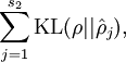
is summing over the hidden units in our network. If you are familiar with the concept of KL divergence, this penalty term is based on it, and can also be written
where
is the Kullback-Leibler (KL) divergence between a Bernoulli random variable with mean
and a Bernoulli random variable with mean
. KL-divergence is a standard function for measuring how different two different distributions are.
偏离,惩罚
 deviating significantly from
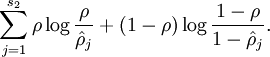
 is the Kullback-Leibler (KL) divergence between a Bernoulli random variable with mean
 损失函数
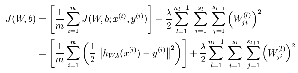
无稀疏约束时网络的损失函数表达式如下:
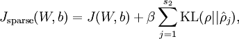
带稀疏约束的损失函数如下:
where
is as defined previously, and
controls the weight of the sparsity penalty term. The term
(implicitly) depends on
also, because it is the average activation of hidden unit
, and the activation of a hidden unit depends on the parameters
.
 is as defined previously, and
  controls the weight of the sparsity penalty term. The term
  also, because it is the average activation of hidden unit
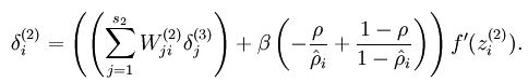
损失函数的偏导数的求法
而加入了稀疏性后,神经元节点的误差表达式由公式:
变成公式:
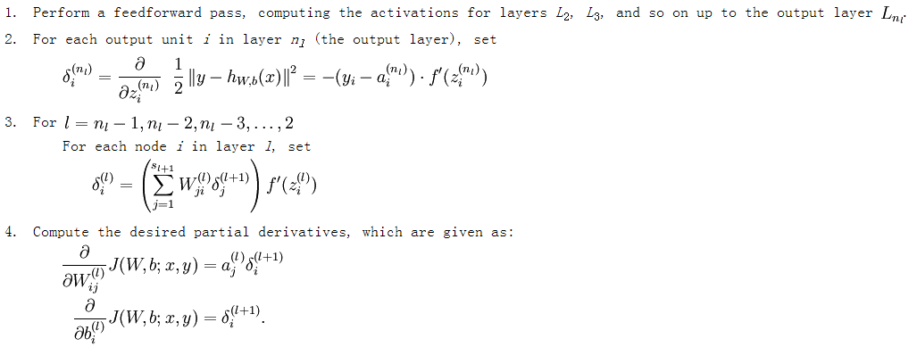

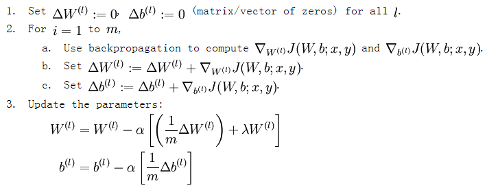
梯度下降法求解
有了损失函数及其偏导数后就可以采用梯度下降法来求网络最优化的参数了,整个流程如下所示:
从上面的公式可以看出,损失函数的偏导其实是个累加过程,每来一个样本数据就累加一次。这是因为损失函数本身就是由每个训练样本的损失叠加而成的,而按照加法的求导法则,损失函数的偏导也应该是由各个训练样本所损失的偏导叠加而成。从这里可以看出,训练样本输入网络的顺序并不重要,因为每个训练样本所进行的操作是等价的,后面样本的输入所产生的结果并不依靠前一次输入结果(只是简单的累加而已,而这里的累加是顺序无关的)。
转自:http://www.cnblogs.com/tornadomeet/archive/2013/03/19/2970101.html

 浙公网安备 33010602011771号