【Stefano M. Iacus】Racon-Nikodym Derivative and MC

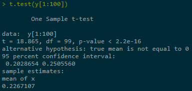
1. Task: Use MC to estimate EY using 100000 replications and construct 95% CI (P(|Z| < 1.96) ≈ 0.95, i.e., 95% of time EY in this interval, e.g., Z = dÃ/dA, reassigning probabilities to the elements in Ω).

set.seed(123)
n <- 100000
beta <- 5
x <- rnorm(n) #X ~ N(0,1)
y <- exp(beta * x)

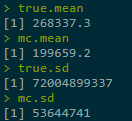
The true sd = 72004899337 is to big with respect to EY. Monte Carlo interval is not informative if variance of Y = g(X) is too large.

true.mean <- exp(beta^2 / 2) # analytical value
true.mean
mc.mean <- mean(y)
mc.mean
true.sd <- sqrt(exp(2 * beta^2) - exp(beta^2))
true.sd
mc.sd <- sd(y)
mc.sd

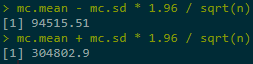
 MC's CI below is based on estimated σ, and it is very big. 

mc.mean - mc.sd * 1.96 / sqrt(n)
mc.mean + mc.sd * 1.96 / sqrt(n)

CI based on true σ is way too much located as bigger values:

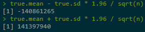
And MC's CI even didn't cover the min value.Reasons: (1) underastimated σ; (2) big variance of g(X) itself; (3) asymptotic normality after 100000 replications is not yet reached (function is exponentially growing). 

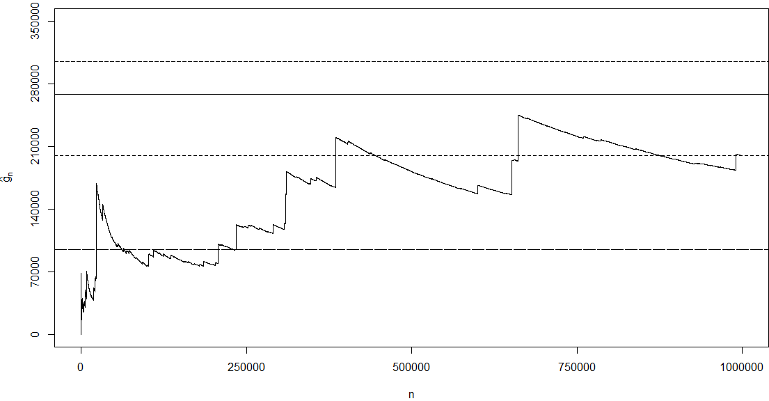
plot(1:n, cumsum(y)/(1:n), type = 'l', axes = F, xlab = 'n',
     ylab = expression(hat(g)[n]), ylim = c(0, 350000))
axis(1, seq(0, n, length = 5))
axis(2, seq(0, 350000, length = 6))
abline(h = 268337.3) # true mean
abline(h = mc.mean - mc.sd * 1.96 / sqrt(n), lty = 3)
abline(h = mc.mean + mc.sd * 1.96 / sqrt(n), lty = 3)
abline(h = mc.mean, lty = 2) # mc estimate 199659.2
box()

2. Calibration (Variance Reduction)

2.1 Preferential Sampling

Task: Calculate Eg(X) with g(X) = max(0, K - e^βx), X ~ N(0,1)

The explicit solution of this put option price p(X) under BS framework:

 Φ is cumulative distribution func, i.e., Φ(x) = P(Z < z) with Z ~ N(0,1).

2.1.1 Without applying var-reduction technique

set.seed(123)
n <- 10000
beta <- 1
K <- 1
x <- rnorm(n) #X ~ N(0,1)
y <- sapply(x, function(x) max(0, K - exp(beta * x))) # vector-wise func
# explicit true solution
K * pnorm(log(K) / beta) - exp(beta^2 / 2) * pnorm(log(K) / beta - beta)

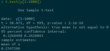
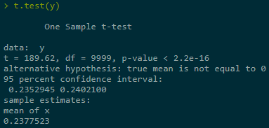
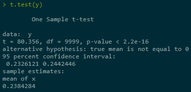
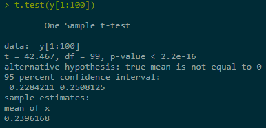
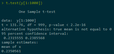
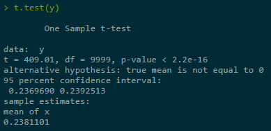
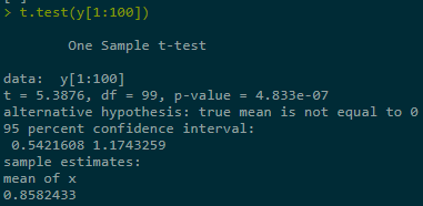
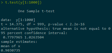
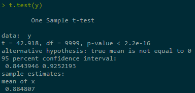
Estimate + construct CI for Y = Eg(X) in three ranges of simulations, last one best:

  

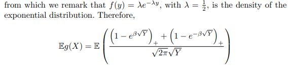
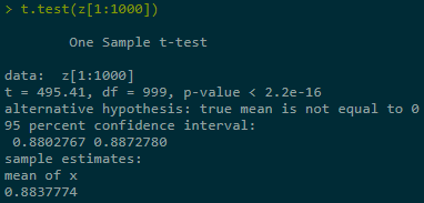
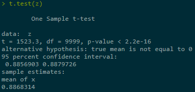
 2.1.2 With applying var-reduction technique

Rewrite Eg(X) as Eg'(X).

Assume K = 1, and e^x - 1≈  x for x → 0, then Eg(X):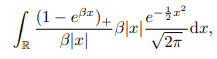 

 Change x = √y, for x > 0; x = -√y, for x < 0, then above equals: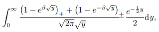 

set.seed(123)
n <- 10000
beta <- 1
K <- 1
x <- rexp(n, rate = 0.5)
h <- function(x) (max(0, 1 - exp(beta * sqrt(x))) +
                          max(0, 1 - exp(-beta * sqrt(x)))) / sqrt(2 * pi * x)
y <- sapply(x, h)

  

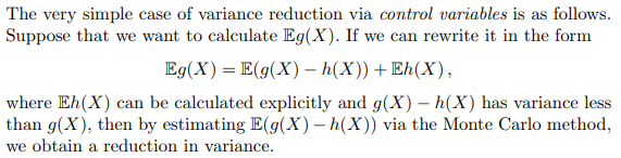
2.2 Control Variables

2.2.1 Task: Task: Calculate Eg(X) with g(X) = max(0, e^βx - K), X ~ N(0,1)

The explicit solution of this call option price c(X) under BS framework: 

Put-call Parity: , where var[c(X)] > var[p(X)].

2.2.2 Without technique

y <- sapply(x, function(x) max(0, exp(beta * x) - K))
exp(beta^2 / 2) * pnorm(beta - log(K) / beta) - K * pnorm(-log(K) / beta)

  2.2.2 With technique

x <- rexp(n, rate = 0.5)
h <- function(x) (max(0, 1 - exp(beta * sqrt(x))) +
                          max(0, 1 - exp(-beta * sqrt(x)))) / sqrt(2 * pi * x)
y <- sapply(x, h)
# CALL = PUT + e^(0.5 * beta^2) - K
z <- y + exp(0.5 * beta^2) - K

  2.3 Antithetic (对偶) Sampling

 

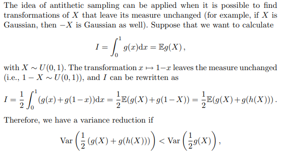
This also means: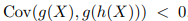 

2.3.1 Task: Calculate p(X) using X and -X, then averaging:

y1 <- sapply(x, function(x) max(0, K - exp(beta * x)))
y2 <- sapply(-x, function(x) max(0, K - exp(beta * x)))
y <- (y1 + y2) / 2
# True value
K * pnorm(log(K) / beta) - exp(beta^2 / 2) * pnorm(log(K) / beta - beta)