机器学习(Machine Learning)- 吴恩达(Andrew Ng) 学习笔记(十四)
Dimensionality Reduction 降维
Motivation I: Data Compression
数据压缩不仅可以节省内存空间,有时也会加快我们的学习算法。
Data compression
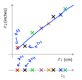
将二维数据压缩到一维,如:数据冗余的情况(横坐标为cm,纵坐标为inches);横纵坐标成某种相关关系时(驾驶员的飞行技巧和对飞行的喜欢程度成正相关)。
降维过程:在原数据的图中找到一个包含绝大部分真实数据的线,测量每个样本在线上的位置,在新图中建立对应的新特征。
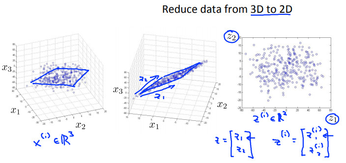
从三维降到二维:将三维的数据投影到一个平面上,使所有点都在这个2D表面。
更典型的例子中可能要从一千维减少到一百维。
Motivation II: Data Visualization
在许多及其学习问题中,如果我们能将数据可视化,以便能寻找到一个更好的解决方案,降维可帮助我们进行数据的可视化。
以下图为例,我们现在有一个关于许多不同国家的数据,每一个特征向量都有50个特征(如GDP,人均GDP,平均寿命等)。
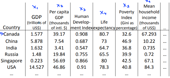
如果要将这个50维的数据可视化,是根本不可能的,使用降维的方法将其降至2维,我们便可以将其可视化了。
这样做的问题在于,降维的算法只负责减少维数,新产生的特征的意义必须由我们自己去发现。
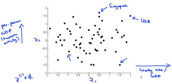
本问题中横坐标为国家GDP,纵坐标为人均GDP或者幸福指数等。图中可理解为:USA国家GDP很大,人均GDP也很大;新加坡国家GDP小一点,人均GDP很大……
Principal Component Analysis problem formulation
针对降维问题,目前最流行、最主流的方法:主成分分析法。
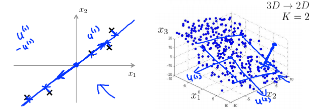
Reduce from 2-dimension to 1-dimension: Find a direction (a vector \(u^{(1)} \in R^n\)) onto which to project the data so as to minimize the projection error.
PCA的目标是将数据从二维降到一维:试着寻找一个属于空间\(R^n\)中的向量\(u^{(i)}\)(一个对数据进行投影的方向),使得投影误差能够最小。
Reduce from n-dimension to k-dimension: Find \(k\) vectors \(u^{(1)},u^{(2)},\dots,u^{(k)}\) onto which to project the data, so as to minimize the project error.
如果是将数据从\(n\)维降到\(k\)维,就要找\(k\)个向量来对数据进行投影。
PCA is not linear regression
主成分分析与线性回归是两种不同的算法。
主成分分析最小化的是投射误差(Projected Error),而线性回归尝试的是最小化预测误差。线性回归的目的是预测结果,而主成分分析不作任何预测。
下图中,左边的是线性回归的误差(垂直于横轴投影),右边则是主要成分分析的误差(垂直于蓝线投影)。
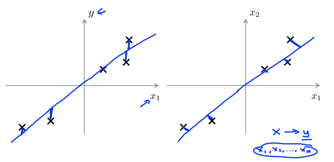
总结:PCA通过寻找一个低维平面对数据进行投影,以便最小化投影误差的平方(每个点与投影后的对应点之间的距离的平方)。
Principal Component Analysis algorithm
Data preprocessing 数据预处理
Training set: \(x^{(1)},x^{(2)},\dots,x^{(m)}\)
Preprocessing (feature scaling/mean normalization): 特征放缩/均值标准化
\(u_j = \frac{1}{m}\sum^m_{i=1}x_j^{(i)}\) 计算每个特征的均值
Replace each \(x_j^{(i)}\) with \(x_j - u_j\). 变量替换
If different features on different scales (e.g., \(x_1\) = size of house, \(x_2\) = number of bedrooms), scale features to have comparable range of values. 如果不同特征对应不同规模,特征放缩使得他们有个相对的取值范围。
PCA algorithm
Reduce data from \(n\)-dimensions to \(k\)-dimensions. Compute "covariance matrix":
Compute "eigenvectors" of matrix \(\Sigma\):
[U, S, V] = svd(Sigma);
进行\(n\)维变量降维到\(k\)维时,需要计算出协方差矩阵,用\(\Sigma\)表示。
From [U, S, V] = svd(Sigma);, we get:
选取\(U\)的前\(K\)列,记为\(U_{reduce}\),为\(n \times k\)维。
令\(Z = U_{reduce}^T x\),得出\(Z\),为\(k \times 1\)维。
After mean normalization (ensure every feature has zero mean) and optionally feature scaling: 为确保均一化后每个特征值都是零均值的,可选特征放缩。
[U, S, V] = svd(Sigma);
Ureduce = U(:,1:k);
z = Ureduce' * x;
Reconstruction for compressed representation
在PCA算法里我们可能需要把1000维的数据压缩为100维的特征向量,或将三维数据压缩到一二维表示。因此,如果这是一种压缩算法,则应该有一种方法可以从这种压缩表示形式返回到原始高维数据的近似值。
因此,给定\(z_i\)(可能为100维),如何返回到原始表示形式\(x_i\)(可能为1000维)?
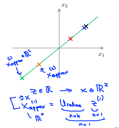
给定一个例子,如下图所示,通过\(z = U_{reduce}^Tx\)得到\(z\)。
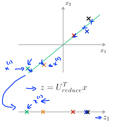
重建原始数据:通过\(x_{approx} = U_{reduce}z\)得到\(x_{approx}\),最终\(x_{approx} \approx x\)。
Choosing the number of principal components
Choosing \(k\) (number of principal components)
Average squared projection error: Total variation in the data:
PCA试图减少投影误差平方的平均值。换句话说,我们希望在平均均方误差与训练集方差的比例尽可能小的情况下选择尽可能小的𝑘值。
Typically, choose \(k\) to be smallest value so that
"99% of variance is retained"
如果我们希望这个比例小于1%,就意味着原本数据的偏差有99%都保留下来了,如果我们选择保留95%的偏差,便能非常显著地降低模型中特征的维度了。
Algorithm:
Try PCA with \(k = 1\)
Compute \(U_{reduce},z^{(1)},z^{(2)},\dots,z^{(m)},x^{(1)}_{approx},\dots,x_{approx}^{(m)}\).
Check if \(\frac{\frac{1}{m}\sum_{i=1}^m||x^{(i)}-x^{(i)}_{approx}||^2}{\frac{1}{m}\sum^m_{i=1}||x^{(i)}||^2}
\le 0.01\).
我们可以先令\(𝑘 = 1\),然后进行主要成分分析,获得\(𝑈_{𝑟𝑒𝑑𝑢𝑐𝑒}\)和\(𝑧\),然后计算比例是否小于1%。
如果不是的话再令\(𝑘 = 2\),如此类推,直到找到可以使得比例小于1%的最小\(𝑘\)值(原因是各个特征之间通常情况存在某种相关性)。
还有一些更好的方式来选择𝑘,当我们在Octave 中调用“svd”函数的时候,我们获得三个参数:
[U, S, V] = svd(sigma)
其中的𝑆是一个\(𝑛 \times 𝑛\)的矩阵,只有对角线上有值,而其它单元都是\(0\),我们可以使用这个矩阵来计算平均均方误差与训练集方差的比例:
即:
在压缩数据后,采取如下方法近似获取原始数据特征:
Advice for applying PCA
Supervised learning speedup
在监督学习算法中,PCA是常被用来加速算法的一个方法。
\((x^{(1)},y^{(1)}),(x^{(2)},y^{(2)}),\dots,(x^{(m)},y^{(m)})\)
Extract inputs:
Unlabeled dataset: \(x^{(1)},x^{(2)},\dots,x^{(m)} \in R^{10000}\)
\(PCA \rightarrow\) \(z^{(1)},z^{(2)},\dots,z^{(m)} \in R^{1000}\)
New training set: \(\{(z^{(1)},y^{(1)}),(z^{(2)},y^{(2)}),\dots,(z^{(m)},y^{(m)})\}\)
每个样本都包括输入\(x\)和标签\(y\),抽取无标签的数据集\(x\),通过PCA算法将它们进行降维操作,得到新的数据集\(z\),用对应的\(z^{(i)}\)代替\(x^{(i)}\)得到新的训练集\((z^{(i)},y^{(i)})\)。
Note: Mapping \(x^{(i)} \rightarrow z^{(i)}\) should be defined by running PCA only on the training set. This mapping can be applied as well to the examples \(x_{cv}^{(i)}\) and \(x_{test}^{(i)}\) in the cross validation and test sets.
注意:在运行PCA时,仅在数据的训练集部分应用。定义了\(x\)到\(z\)的映射后,该映射可应用于交叉验证集和测试集。
Application of PCA
- Compression 通过尝试不同的\(k\)
- Reduce memory/disk needed to stire data
- Speed up learning algorithm
- Visualization \(k = 2\)或\(k = 3\)
Bad use of PCA: To prevent overfitting
Use \(z^{(i)}\) instead of \(x^{(i)}\) to reduce the number of features to \(k \lt n\).
Thus, fewer features, less likely to overfit.
使用PCA来减少特征值的数量,从而防止过拟合的产生,可能不是一个好的方法。采用正则化的方法会好点。因为PCA不使用标签\(y\),仅通过\(x\)来对数据进行低维近似,所以PCA有时会舍掉一些有价值的信息。
This might work OK, but isn't a good way to address overfitting. Use regularization instead.
PCA is sometimes used where it shouldn't be
PCA的“滥用”
Design of ML system:
- Get training set \(\{(x^{(1)},y^{(1)}),(x^{(2)},y^{(2)}),\dots,(x^{(m)},y^{(m)})\}\)
- Run PCA to reduce \(x^{(i)}\) in dimension to get \(z^{(i)}\)
- Train logistic regression on \(\{(z^{(1)},y^{(1)}),(z^{(2)},y^{(2)}),\dots,(z^{(m)},y^{(m)})\}\)
- Test on test set: Map \(x^{(i)}_{test}\) yo \(z^{(i)}_{test}\). Run \(h_\theta(z)\) on \(\{(z^{(1)}_{test}, y^{(1)}_{test}),(z^{(2)}_{test},y^{(2)})_{test},\dots,(z^{(m)}_{test},y^{(m)}_{test})\}\)
How about doing the whole thing without using PCA?
Before implementing PCA, first try running whatever you want to do with the original/raw data \(x^{(i)}\). Only if that doesn't do what you want, then implement PCA and consider using \(z^{(i)}\).
在执行PCA之前,首先尝试用你原始的数据\(x^{(i)}\)进行处理,当该操作不能满足要求时,再考虑实施PCA。
