机器学习-卷积神经网络(pytorch环境)
参考资料
(复制一遍笔记是为了加深印象)
理论基础
Why CNN for Image?
CNN V.s. DNN
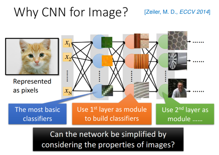
在train neural network的时候,我们会有一种期待说,在这个network structure里面的每一个neuron,都应该代表了一个最基本的classifier;事实上,在文献上,根据训练的结果,也有很多人得到这样的结论,举例来说,下图中:
- 第一个layer的neuron,它就是最简单的classifier,它做的事情就是detect有没有绿色出现、有没有黄色出现、有没有斜的条纹出现等等
- 那第二个layer,它做的事情是detect更复杂的东西,根据第一个layer的output,它如果看到直线横线,就是窗框的一部分;如果看到棕色的直条纹就是木纹;看到斜条纹加灰色的,这个有可能是很多东西,比如说,轮胎的一部分等等
- 再根据第二个hidden layer的output,第三个hidden layer会做更复杂的事情,比如它可以知道说,当某一个neuron看到蜂巢,它就会被activate;当某一个neuron看到车子,它就会被activate;当某一个neuron看到人的上半身,它就会被activate等等
那现在的问题是这样子:当我们直接用一般的fully connected的feedforward network来做图像处理的时候,往往会需要太多的参数
举例来说,假设这是一张100*100的彩色图片,它的分辨率才100*100,那这已经是很小张的image了,然后你需要把它拉成一个vector,总共有100*100*3个pixel(如果是彩色的图的话,每个pixel其实需要3个value,即RGB值来描述它的),把这些加起来input vectot就已经有三万维了;如果input vector是三万维,又假设hidden layer有1000个neuron,那仅仅是第一层hidden layer的参数就已经有30000*1000个了,这样就太多了
所以,CNN做的事情其实是,来简化这个neural network的架构,我们根据自己的知识和对图像处理的理解,一开始就把某些实际上用不到的参数给过滤掉,我们一开始就想一些办法,不要用fully connected network,而是用比较少的参数,来做图像处理这件事情,所以CNN其实是比一般的DNN还要更简单的
虽然CNN看起来,它的运作比较复杂,但事实上,它的模型比DNN还要更简单,我们就是用prior knowledge,去把原来fully connected的layer里面的一些参数拿掉,就变成CNN
为什么我们有可能把一些参数拿掉?为什么我们有可能只用比较少的参数就可以来做图像处理这件事情?下面列出三个对影像处理的观察:(这也是CNN架构提出的基础所在!!!)
Some patterns are much smaller than the whole image
在影像处理里面,如果在network的第一层hidden layer里,那些neuron要做的事情是侦测有没有一种东西、一种pattern(图案样式)出现,那大部分的pattern其实是比整张image要小的,所以对一个neuron来说,想要侦测有没有某一个pattern出现,它其实并不需要看整张image,只需要看这张image的一小部分,就可以决定这件事情了
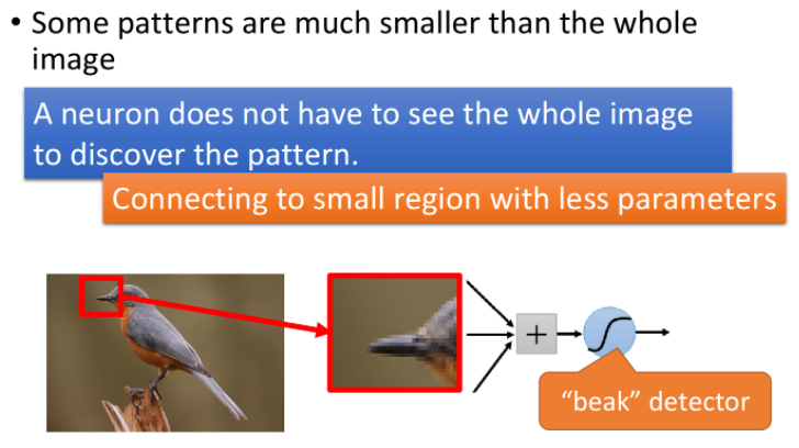
举例来说,假设现在我们有一张鸟的图片,那第一层hidden layer的某一个neuron的工作是,检测有没有鸟嘴的存在(你可能还有一些neuron侦测有没有鸟嘴的存在、有一些neuron侦测有没有爪子的存在、有一些neuron侦测有没有翅膀的存在、有没有尾巴的存在,之后合起来,就可以侦测,图片中有没有一只鸟),那它其实并不需要看整张图,因为,其实我们只要给neuron看这个小的红色杠杠里面的区域,它其实就可以知道说,这是不是一个鸟嘴,对人来说也是一样,只要看这个小的区域你就会知道说这是鸟嘴,所以,每一个neuron其实只要连接到一个小块的区域就好,它不需要连接到整张完整的图,因此也对应着更少的参数
The same patterns appear in different regions
同样的pattern,可能会出现在image的不同部分,但是它们有同样的形状、代表的是同样的含义,因此它们也可以用同样的neuron、同样的参数,被同一个detector检测出来
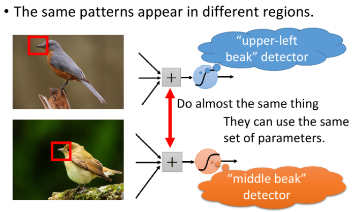
举例来说,上图中分别有一个处于左上角的鸟嘴和一个处于中央的鸟嘴,但你并不需要训练两个不同的detector去专门侦测左上角有没有鸟嘴和中央有没有鸟嘴这两件事情,这样做太冗余了,我们要cost down(降低成本),我们并不需要有两个neuron、两组不同的参数来做duplicate(重复一样)的事情,所以我们可以要求这些功能几乎一致的neuron共用一组参数,它们share同一组参数就可以帮助减少总参数的量
Subsampling the pixels will not change the object
我们可以对一张image做subsampling(二次抽样),假如你把它奇数行、偶数列的pixel拿掉,image就可以变成原来的十分之一大小,而且并不会影响人对这张image的理解,对你来说,下面两张大小不一的image看起来不会有什么太大的区别,你都可以识别里面有什么物件,因此subsampling对图像辨识来说,可能是没有太大的影响的
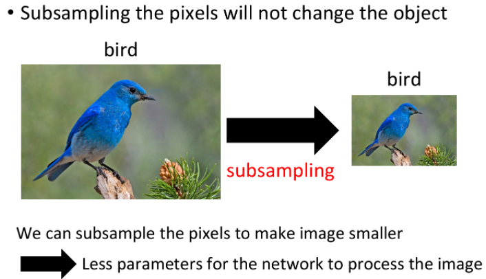
所以,我们可以利用subsampling这个概念把image变小,从而减少需要用到的参数量
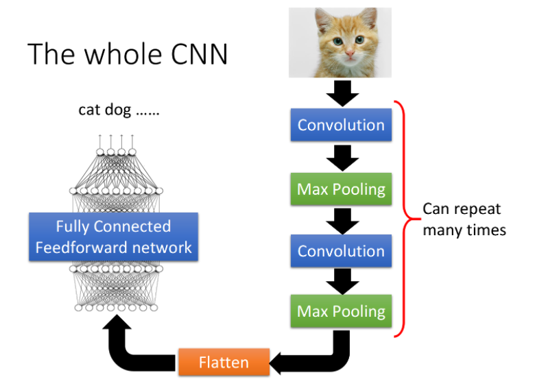
The whole CNN structure
整个CNN的架构是这样的:
首先,input一张image以后,它会先通过Convolution的layer,接下来做Max Pooling这件事,然后再去做Convolution,再做Maxi Pooling...,这个process可以反复进行多次(重复次数需要事先决定),这就是network的架构,就好像network有几层一样,你要做几次convolution,做几次Max Pooling,在定这个network的架构时就要事先决定好
当你做完先前决定的convolution和max pooling的次数后,你要做的事情是Flatten,做完flatten以后,你就把Flatten output丢到一般的Fully connected network里面去,最终得到影像辨识的结果
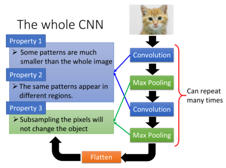
我们基于之前提到的三个对影像处理的观察,设计了CNN这样的架构,第一个是要侦测一个pattern,你不需要看整张image,只要看image的一个小部分;第二个是同样的pattern会出现在一张图片的不同区域;第三个是我们可以对整张image做subsampling
那前面这两个property,是用convolution的layer来处理的;最后这个property,是用max pooling来处理的
Convolution
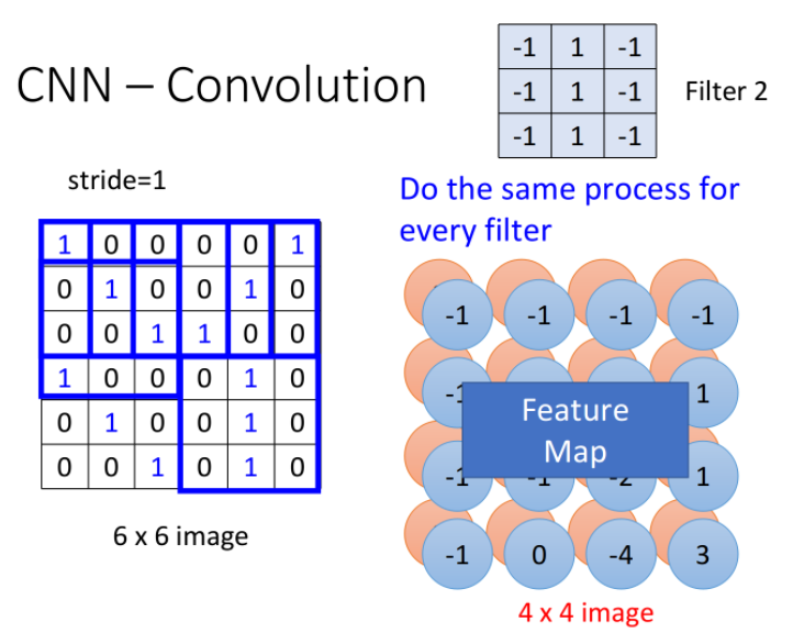
假设现在我们network的input是一张6*6的image,图像是黑白的,因此每个pixel只需要用一个value来表示,而在convolution layer里面,有一堆Filter,这边的每一个Filter,其实就等同于是Fully connected layer里的一个neuron
Property 1
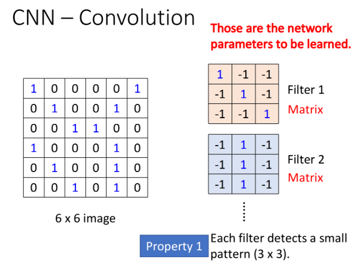
每一个Filter其实就是一个matrix,这个matrix里面每一个element的值,就跟那些neuron的weight和bias一样,是network的parameter,它们具体的值都是通过Training data学出来的,而不是人去设计的
所以,每个Filter里面的值是什么,要做什么事情,都是自动学习出来的,上图中每一个filter是3*3的size,意味着它就是在侦测一个3*3的pattern,当它侦测的时候,并不会去看整张image,它只看一个3*3范围内的pixel,就可以判断某一个pattern有没有出现,这就考虑了property 1
Property 2
这个filter是从image的左上角开始,做一个slide window,每次向右挪动一定的距离,这个距离就叫做stride,由你自己设定,每次filter停下的时候就跟image中对应的3*3的matrix做一个内积(相同位置的值相乘并累计求和),这里假设stride=1,那么我们的filter每次移动一格,当它碰到image最右边的时候,就从下一行的最左边开始重复进行上述操作,经过一整个convolution的process,最终得到下图所示的红色的4*4 matrix
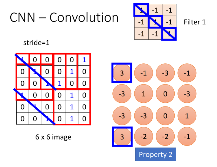
观察上图中的Filter1,它斜对角的地方是1,1,1,所以它的工作就是detect有没有连续的从左上角到右下角的1,1,1出现在这个image里面,检测到的结果已在上图中用蓝线标识出来,此时filter得到的卷积结果的左上和左下得到了最大的值,这就代表说,该filter所要侦测的pattern出现在image的左上角和左下角
同一个pattern出现在image左上角的位置和左下角的位置,并不需要用到不同的filter,我们用filter1就可以侦测出来,这就考虑了property 2
Feature Map
在一个convolution的layer里面,它会有一打filter,不一样的filter会有不一样的参数,但是这些filter做卷积的过程都是一模一样的,你把filter2跟image做完convolution以后,你就会得到另外一个蓝色的4*4 matrix,那这个蓝色的4*4 matrix跟之前红色的4*4matrix合起来,就叫做Feature Map(特征映射),有多少个filter,对应就有多少个映射后的image
CNN对不同scale的相同pattern的处理上存在一定的困难,由于现在每一个filter size都是一样的,这意味着,如果你今天有同一个pattern,它有不同的size,有大的鸟嘴,也有小的鸟嘴,CNN并不能够自动处理这个问题;DeepMind曾经发过一篇paper,上面提到了当你input一张image的时候,它在CNN前面,再接另外一个network,这个network做的事情是,它会output一些scalar,告诉你说,它要把这个image的里面的哪些位置做旋转、缩放,然后,再丢到CNN里面,这样你其实会得到比较好的performance
Colorful image
刚才举的例子是黑白的image,所以你input的是一个matrix,如果今天是彩色的image会怎么样呢?我们知道彩色的image就是由RGB组成的,所以一个彩色的image,它就是好几个matrix叠在一起,是一个立方体,如果我今天要处理彩色的image,要怎么做呢?
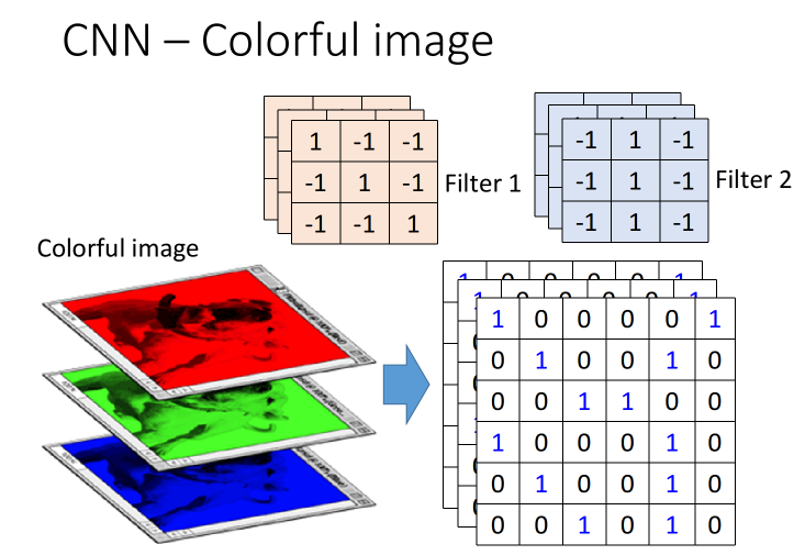
这个时候你的filter就不再是一个matrix了,它也会是一个立方体,如果你今天是RGB这三个颜色来表示一个pixel的话,那你的input就是3*6*6,你的filter就是3*3*3,你的filter的高就是3,你在做convolution的时候,就是把这个filter的9个值跟这个image里面的9个值做内积,可以想象成filter的每一层都分别跟image的三层做内积,得到的也是一个三层的output,每一个filter同时就考虑了不同颜色所代表的channel
Convolution V.s. Fully connected
filter是特殊的”neuron“
接下来要讲的是,convolution跟fully connected有什么关系,你可能觉得说,它是一个很特别的operation,感觉跟neural network没半毛钱关系,其实,它就是一个neural network
convolution这件事情,其实就是fully connected的layer把一些weight拿掉而已,下图中绿色方框标识出的feature map的output,其实就是hidden layer的neuron的output

接下来我们来解释这件事情:
如下图所示,我们在做convolution的时候,把filter放在image的左上角,然后再去做inner product,得到一个值3;这件事情等同于,我们现在把这个image的6*6的matrix拉直变成右边这个用于input的vector,然后,你有一个红色的neuron,这些input经过这个neuron之后,得到的output是3

每个“neuron”只检测image的部分区域
那这个neuron的output怎么来的呢?这个neuron实际上就是由filter转化而来的,我们把filter放在image的左上角,此时filter考虑的就是和它重合的9个pixel,假设你把这一个6*6的image的36个pixel拉成直的vector作为input,那这9个pixel分别就对应着右侧编号1,2,3的pixel,编号7,8,9的pixel跟编号13,14,15的pixel
如果我们说这个filter和image matrix做inner product以后得到的output 3,就是input vector经过某个neuron得到的output 3的话,这就代表说存在这样一个neuron,这个neuron带weight的连线,就只连接到编号为1,2,3,7,8,9,13,14,15的这9个pixel而已,而这个neuron和这9个pixel连线上所标注的的weight就是filter matrix里面的这9个数值
作为对比,Fully connected的neuron是必须连接到所有36个input上的,但是,我们现在只用连接9个input,因为我们知道要detect一个pattern,不需要看整张image,看9个input pixel就够了,所以当我们这么做的时候,就用了比较少的参数
“neuron”之间共享参数
当我们把filter做stride = 1的移动的时候,会发生什么事呢?此时我们通过filter和image matrix的内积得到另外一个output值-1,我们假设这个-1是另外一个neuron的output,那这个neuron会连接到哪些input呢?下图中这个框起来的地方正好就对应到pixel 2,3,4,pixel 8,9,10跟pixel 14,15,16

你会发现output为3和-1的这两个neuron,它们分别去检测在image的两个不同位置上是否存在某个pattern,因此在Fully connected layer里它们做的是两件不同的事情,每一个neuron应该有自己独立的weight
但是,当我们做这个convolution的时候,首先我们把每一个neuron前面连接的weight减少了,然后我们强迫某些neuron(比如上图中output为3和-1的两个neuron),它们一定要共享一组weight,虽然这两个neuron连接到的pixel对象各不相同,但它们用的weight都必须是一样的,等于filter里面的元素值,这件事情就叫做weight share,当我们做这件事情的时候,用的参数,又会比原来更少
总结
因此我们可以这样想,有这样一些特殊的neuron,它们只连接着9条带weight的线(9=3*3对应着filter的元素个数,这些weight也就是filter内部的元素值,上图中圆圈的颜色与连线的颜色一一对应)
当filter在image matrix上移动做convolution的时候,每次移动做的事情实际上是去检测这个地方有没有某一种pattern,对于Fully connected layer来说,它是对整张image做detection的,因此每次去检测image上不同地方有没有pattern其实是不同的事情,所以这些neuron都必须连接到整张image的所有pixel上,并且不同neuron的连线上的weight都是相互独立的
那对于convolution layer来说,首先它是对image的一部分做detection的,因此它的neuron只需要连接到image的部分pixel上,对应连线所需要的weight参数就会减少;其次由于是用同一个filter去检测不同位置的pattern,所以这对convolution layer来说,其实是同一件事情,因此不同的neuron,虽然连接到的pixel对象各不相同,但是在“做同一件事情”的前提下,也就是用同一个filter的前提下,这些neuron所使用的weight参数都是相同的,通过这样一张weight share的方式,再次减少network所需要用到的weight参数
CNN的本质,就是减少参数的过程
补充
看到这里你可能会问,这样的network该怎么搭建,又该怎么去train呢?
首先,第一件事情就是这都是用toolkit做的,所以你大概不会自己去写;如果你要自己写的话,它其实就是跟原来的Backpropagation用一模一样的做法,只是有一些weight就永远是0,你就不去train它,它就永远是0
然后,怎么让某些neuron的weight值永远都是一样呢?你就用一般的Backpropagation的方法,对每个weight都去算出gradient,再把本来要tight在一起、要share weight的那些weight的gradient平均,然后,让他们update同样值就ok了
Max Pooling
Operation of max pooling
相较于convolution,max pooling是比较简单的,它就是做subsampling,根据filter 1,我们得到一个4*4的matrix,根据filter 2,你得到另外一个4*4的matrix,接下来,我们要做什么事呢?
我们把output四个分为一组,每一组里面通过选取平均值或最大值的方式,把原来4个value合成一个 value,这件事情相当于在image每相邻的四块区域内都挑出一块来检测,这种subsampling的方式就可以让你的image缩小!

讲到这里你可能会有一个问题,如果取Maximum放到network里面,不就没法微分了吗?max这个东西,感觉是没有办法对它微分的啊,其实是可以的,后面的章节会讲到Maxout network,会告诉你怎么用微分的方式来处理它
Convolution + Max Pooling
所以,结论是这样的:
做完一次convolution加一次max pooling,我们就把原来6*6的image,变成了一个2*2的image;至于这个2*2的image,它每一个pixel的深度,也就是每一个pixel用几个value来表示,就取决于你有几个filter,如果你有50个filter,就是50维,像下图中是两个filter,对应的深度就是两维
所以,这是一个新的比较小的image,它表示的是不同区域上提取到的特征,实际上不同的filter检测的是该image同一区域上的不同特征属性,所以每一层channel(通道)代表的是一种属性,一块区域有几种不同的属性,就有几层不同的channel,对应的就会有几个不同的filter对其进行convolution操作

这件事情可以repeat很多次,你可以把得到的这个比较小的image,再次进行convolution和max pooling的操作,得到一个更小的image,依次类推
有这样一个问题:假设我第一个convolution有25个filter,通过这些filter得到25个feature map,然后repeat的时候第二个convolution也有25个filter,那这样做完,我是不是会得到25^2个feature map?
其实不是这样的,你这边做完一次convolution,得到25个feature map之后再做一次convolution,还是会得到25个feature map,因为convolution在考虑input的时候,是会考虑深度的,它并不是每一个channel分开考虑,而是一次考虑所有的channel,所以,你convolution这边有多少个filter,再次output的时候就会有多少个channel
因此你这边有25个channel,经过含有25个filter的convolution之后output还会是25个channel,只是这边的每一个channel,它都是一个cubic(立方体),它的高有25个value那么高

Flatten
做完convolution和max pooling之后,就是FLatten和Fully connected Feedforward network的部分
Flatten的意思是,把左边的feature map拉直,然后把它丢进一个Fully connected Feedforward network,然后就结束了,也就是说,我们之前通过CNN提取出了image的feature,它相较于原先一整个image的vetor,少了很大一部分内容,因此需要的参数也大幅度地减少了,但最终,也还是要丢到一个Fully connected的network中去做最后的分类工作

代码实践
神经网络基本骨架
import torch
from torch import nn

class TuDui(nn.Module):
    def __init__(self):
        super().__init__()

    def forward(self,input):
        output = input + 1
        return output

tudui = TuDui()
x = torch.tensor(1.0)
output = tudui(x)
print(output)


class Module:
    r"""Base class for all neural network modules.

    Your models should also subclass this class.

    Modules can also contain other Modules, allowing to nest them in
    a tree structure. You can assign the submodules as regular attributes::

        import torch.nn as nn
        import torch.nn.functional as F

        class Model(nn.Module):
            def __init__(self):
                super(Model, self).__init__()
                self.conv1 = nn.Conv2d(1, 20, 5)
                self.conv2 = nn.Conv2d(20, 20, 5)

            def forward(self, x):
                x = F.relu(self.conv1(x))
                return F.relu(self.conv2(x))

    Submodules assigned in this way will be registered, and will have their
    parameters converted too when you call :meth:`to`, etc.

    :ivar training: Boolean represents whether this module is in training or
                    evaluation mode.
    :vartype training: bool
    """
Conv2d
一个列子
import torch
import torchvision.datasets
from torch import nn
from torch.nn import Conv2d
from torch.utils.data import DataLoader
from torch.utils.tensorboard import SummaryWriter

dataset_transform = torchvision.transforms.Compose([
    torchvision.transforms.ToTensor()
])

dataset = torchvision.datasets.CIFAR10(root='./dataset', train=False, transform=dataset_transform, download=True)

writer = SummaryWriter("conv2d")

dataLoader = DataLoader(dataset=dataset, batch_size=64, shuffle=True, num_workers=0, drop_last=False)

class TuDui(nn.Module):
    def __init__(self):
        super(TuDui, self).__init__()
        self.conv1 = Conv2d(in_channels=3,out_channels=6,kernel_size=3,stride=1,padding=0)

    def forward(self,x):
        x = self.conv1(x)
        return x

tudui = TuDui()
step = 0
for data in dataLoader:
    # 输入三通道
    imgs, targets = data
    # 输出六通道
    output = tudui(imgs)
    writer.add_images("input",imgs,step)
    # 变换
    output = torch.reshape(output, (-1, 3, 30, 30))
    writer.add_images("output",output,step)
    step += 1

writer.close()
为什么要做变换?
因为输出的数据是六个通道,如果想要显示3通道的图片,就需要把6通道的输出分开,使用torch.reshape()方法
torch.reshape(input, shape) → Tensor
Returns a tensor with the same data and number of elements as input, but with the specified shape. When possible, the returned tensor will be a view of input. Otherwise, it will be a copy. Contiguous inputs and inputs with compatible strides can be reshaped without copying, but you should not depend on the copying vs. viewing behavior.

See torch.Tensor.view() on when it is possible to return a view.

A single dimension may be -1, in which case it’s inferred from the remaining dimensions and the number of elements in input.

Parameters
input (Tensor) – the tensor to be reshaped

shape (tuple of python:ints) – the new shape
其中(-1,3,30,30)中的-1表示由程序计算出,3表示输出为3通道,30,30为输出图片的大小
MaxPool2d
一个例子:
import torch
import torchvision.datasets
from torch import nn
from torch.nn import Conv2d, MaxPool2d
from torch.utils.data import DataLoader
from torch.utils.tensorboard import SummaryWriter

dataset_transform = torchvision.transforms.Compose([
    torchvision.transforms.ToTensor()
])

dataset = torchvision.datasets.CIFAR10(root='./dataset', train=False, transform=dataset_transform, download=True)

writer = SummaryWriter("maxPool2d")

dataLoader = DataLoader(dataset=dataset, batch_size=1, shuffle=True, num_workers=0, drop_last=False)

class TuDui(nn.Module):
    def __init__(self):
        super(TuDui, self).__init__()
        self.maxpool = MaxPool2d(kernel_size=3, ceil_mode=False)

    def forward(self,x):
        x = self.maxpool(x)
        return x

tudui = TuDui()
step = 0
for data in dataLoader:
    imgs, targets = data
    output = tudui(imgs)
    writer.add_images("input",imgs,step)
    writer.add_images("output",output,step)
    step += 1

writer.close()
class MaxPool2d(_MaxPoolNd):
    r"""Applies a 2D max pooling over an input signal composed of several input
    planes.

    In the simplest case, the output value of the layer with input size :math:`(N, C, H, W)`,
    output :math:`(N, C, H_{out}, W_{out})` and :attr:`kernel_size` :math:`(kH, kW)`
    can be precisely described as:

    .. math::
        \begin{aligned}
            out(N_i, C_j, h, w) ={} & \max_{m=0, \ldots, kH-1} \max_{n=0, \ldots, kW-1} \\
                                    & \text{input}(N_i, C_j, \text{stride[0]} \times h + m,
                                                   \text{stride[1]} \times w + n)
        \end{aligned}

    If :attr:`padding` is non-zero, then the input is implicitly zero-padded on both sides
    for :attr:`padding` number of points. :attr:`dilation` controls the spacing between the kernel points.
    It is harder to describe, but this `link`_ has a nice visualization of what :attr:`dilation` does.

    Note:
        When ceil_mode=True, sliding windows are allowed to go off-bounds if they start within the left padding
        or the input. Sliding windows that would start in the right padded region are ignored.

    The parameters :attr:`kernel_size`, :attr:`stride`, :attr:`padding`, :attr:`dilation` can either be:

        - a single ``int`` -- in which case the same value is used for the height and width dimension
        - a ``tuple`` of two ints -- in which case, the first `int` is used for the height dimension,
          and the second `int` for the width dimension

    Args:
        kernel_size: the size of the window to take a max over
        stride: the stride of the window. Default value is :attr:`kernel_size`
        padding: implicit zero padding to be added on both sides
        dilation: a parameter that controls the stride of elements in the window
        return_indices: if ``True``, will return the max indices along with the outputs.
                        Useful for :class:`torch.nn.MaxUnpool2d` later
        ceil_mode: when True, will use `ceil` instead of `floor` to compute the output shape

    Shape:
        - Input: :math:`(N, C, H_{in}, W_{in})`
        - Output: :math:`(N, C, H_{out}, W_{out})`, where

          .. math::
              H_{out} = \left\lfloor\frac{H_{in} + 2 * \text{padding[0]} - \text{dilation[0]}
                    \times (\text{kernel\_size[0]} - 1) - 1}{\text{stride[0]}} + 1\right\rfloor

          .. math::
              W_{out} = \left\lfloor\frac{W_{in} + 2 * \text{padding[1]} - \text{dilation[1]}
                    \times (\text{kernel\_size[1]} - 1) - 1}{\text{stride[1]}} + 1\right\rfloor

    Examples::

        >>> # pool of square window of size=3, stride=2
        >>> m = nn.MaxPool2d(3, stride=2)
        >>> # pool of non-square window
        >>> m = nn.MaxPool2d((3, 2), stride=(2, 1))
        >>> input = torch.randn(20, 16, 50, 32)
        >>> output = m(input)

    .. _link:
        https://github.com/vdumoulin/conv_arithmetic/blob/master/README.md
    """