Numpy和数据展示的可视化介绍

 

 

https://jalammar.github.io/visual-numpy/

 

 

http://www.junphy.com/wordpress/index.php/2019/10/24/visual-numpy/

 

A Visual Intro to NumPy and Data Representation

Discussions: Hacker News (366 points, 21 comments), Reddit r/MachineLearning (256 points, 18 comments)
Translations: Chinese 1, Chinese 2, Japanese, Korean

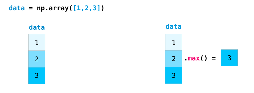
The NumPy package is the workhorse of data analysis, machine learning, and scientific computing in the python ecosystem. It vastly simplifies manipulating and crunching vectors and matrices. Some of python’s leading package rely on NumPy as a fundamental piece of their infrastructure (examples include scikit-learn, SciPy, pandas, and tensorflow). Beyond the ability to slice and dice numeric data, mastering numpy will give you an edge when dealing and debugging with advanced usecases in these libraries.

In this post, we’ll look at some of the main ways to use NumPy and how it can represent different types of data (tables, images, text…etc) before we can serve them to machine learning models.

import numpy as np

Creating Arrays

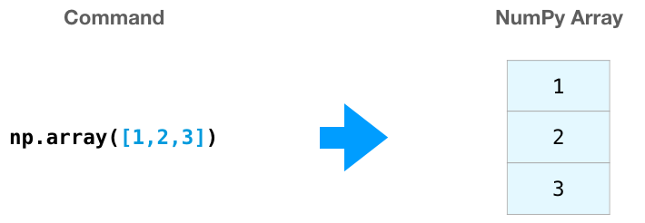
We can create a NumPy array (a.k.a. the mighty ndarray) by passing a python list to it and using ` np.array()`. In this case, python creates the array we can see on the right here:

There are often cases when we want NumPy to initialize the values of the array for us. NumPy provides methods like ones(), zeros(), and random.random() for these cases. We just pass them the number of elements we want it to generate:

Once we’ve created our arrays, we can start to manipulate them in interesting ways.

Array Arithmetic

Let’s create two NumPy arrays to showcase their usefulness. We’ll call them data and ones:

 

Adding them up position-wise (i.e. adding the values of each row) is as simple as typing data + ones:

 

When I started learning such tools, I found it refreshing that an abstraction like this makes me not have to program such a calculation in loops. It’s a wonderful abstraction that allows you to think about problems at a higher level.

And it’s not only addition that we can do this way:

 

There are often cases when we want to carry out an operation between an array and a single number (we can also call this an operation between a vector and a scalar). Say, for example, our array represents distance in miles, and we want to convert it to kilometers. We simply say data * 1.6:

 

See how NumPy understood that operation to mean that the multiplication should happen with each cell? That concept is called broadcasting, and it’s very useful.

Indexing

We can index and slice NumPy arrays in all the ways we can slice python lists:

Aggregation

Additional benefits NumPy gives us are aggregation functions:

In addition to min, max, and sum, you get all the greats like mean to get the average, prod to get the result of multiplying all the elements together, std to get standard deviation, and plenty of others.

In more dimensions

All the examples we’ve looked at deal with vectors in one dimension. A key part of the beauty of NumPy is its ability to apply everything we’ve looked at so far to any number of dimensions.

Creating Matrices

We can pass python lists of lists in the following shape to have NumPy create a matrix to represent them:

np.array([[1,2],[3,4]])

We can also use the same methods we mentioned above (ones(), zeros(), and random.random()) as long as we give them a tuple describing the dimensions of the matrix we are creating:

 

Matrix Arithmetic

We can add and multiply matrices using arithmetic operators (+-*/) if the two matrices are the same size. NumPy handles those as position-wise operations:

 

We can get away with doing these arithmetic operations on matrices of different size only if the different dimension is one (e.g. the matrix has only one column or one row), in which case NumPy uses its broadcast rules for that operation:

 

Dot Product

A key distinction to make with arithmetic is the case of matrix multiplication using the dot product. NumPy gives every matrix a dot() method we can use to carry-out dot product operations with other matrices:

 

I’ve added matrix dimensions at the bottom of this figure to stress that the two matrices have to have the same dimension on the side they face each other with. You can visualize this operation as looking like this:

Matrix Indexing

Indexing and slicing operations become even more useful when we’re manipulating matrices:

 

Matrix Aggregation

We can aggregate matrices the same way we aggregated vectors:

 

Not only can we aggregate all the values in a matrix, but we can also aggregate across the rows or columns by using the axis parameter:

 

Transposing and Reshaping

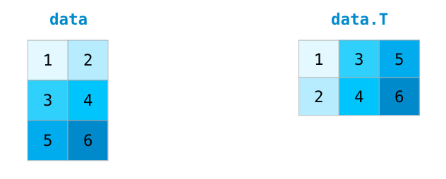
A common need when dealing with matrices is the need to rotate them. This is often the case when we need to take the dot product of two matrices and need to align the dimension they share. NumPy arrays have a convenient property called T to get the transpose of a matrix:

 

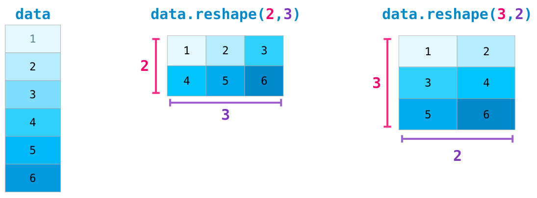
In more advanced use case, you may find yourself needing to switch the dimensions of a certain matrix. This is often the case in machine learning applications where a certain model expects a certain shape for the inputs that is different from your dataset. NumPy’s reshape() method is useful in these cases. You just pass it the new dimensions you want for the matrix. You can pass -1 for a dimension and NumPy can infer the correct dimension based on your matrix:

 

Yet More Dimensions

NumPy can do everything we’ve mentioned in any number of dimensions. Its central data structure is called ndarray (N-Dimensional Array) for a reason.

In a lot of ways, dealing with a new dimension is just adding a comma to the parameters of a NumPy function:

Note: Keep in mind that when you print a 3-dimensional NumPy array, the text output visualizes the array differently than shown here. NumPy’s order for printing n-dimensional arrays is that the last axis is looped over the fastest, while the first is the slowest. Which means that np.ones((4,3,2)) would be printed as:

array([[[1., 1.],
        [1., 1.],
        [1., 1.]],

       [[1., 1.],
        [1., 1.],
        [1., 1.]],

       [[1., 1.],
        [1., 1.],
        [1., 1.]],

       [[1., 1.],
        [1., 1.],
        [1., 1.]]])

Practical Usage

And now for the payoff. Here are some examples of the useful things NumPy will help you through.

Formulas

Implementing mathematical formulas that work on matrices and vectors is a key use case to consider NumPy for. It’s why NumPy is the darling of the scientific python community. For example, consider the mean square error formula that is central to supervised machine learning models tackling regression problems:

 

Implementing this is a breeze in NumPy:

 

The beauty of this is that numpy does not care if predictions and labels contain one or a thousand values (as long as they’re both the same size). We can walk through an example stepping sequentially through the four operations in that line of code:

 

Both the predictions and labels vectors contain three values. Which means n has a value of three. After we carry out the subtraction, we end up with the values looking like this:

 

Then we can square the values in the vector:

 

Now we sum these values:

 

Which results in the error value for that prediction and a score for the quality of the model.

Data Representation

Think of all the data types you’ll need to crunch and build models around (spreadsheets, images, audio…etc). So many of them are perfectly suited for representation in an n-dimensional array:

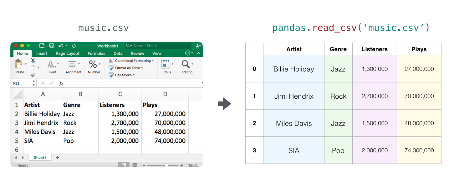
Tables and Spreadsheets

• A spreadsheet or a table of values is a two dimensional matrix. Each sheet in a spreadsheet can be its own variable. The most popular abstraction in python for those is the pandas dataframe, which actually uses NumPy and builds on top of it.

Audio and Timeseries

• An audio file is a one-dimensional array of samples. Each sample is a number representing a tiny chunk of the audio signal. CD-quality audio may have 44,100 samples per second and each sample is an integer between -32767 and 32768. Meaning if you have a ten-seconds WAVE file of CD-quality, you can load it in a NumPy array with length 10 * 44,100 = 441,000 samples. Want to extract the first second of audio? simply load the file into a NumPy array that we’ll call audio, and get audio[:44100].

Here’s a look at a slice of an audio file:

The same goes for time-series data (for example, the price of a stock over time).

Images

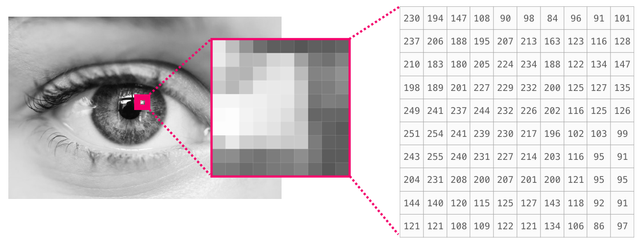
• An image is a matrix of pixels of size (height x width).

  • If the image is black and white (a.k.a. grayscale), each pixel can be represented by a single number (commonly between 0 (black) and 255 (white)). Want to crop the top left 10 x 10 pixel part of the image? Just tell NumPy to get you image[:10,:10].

Here’s a look at a slice of an image file:

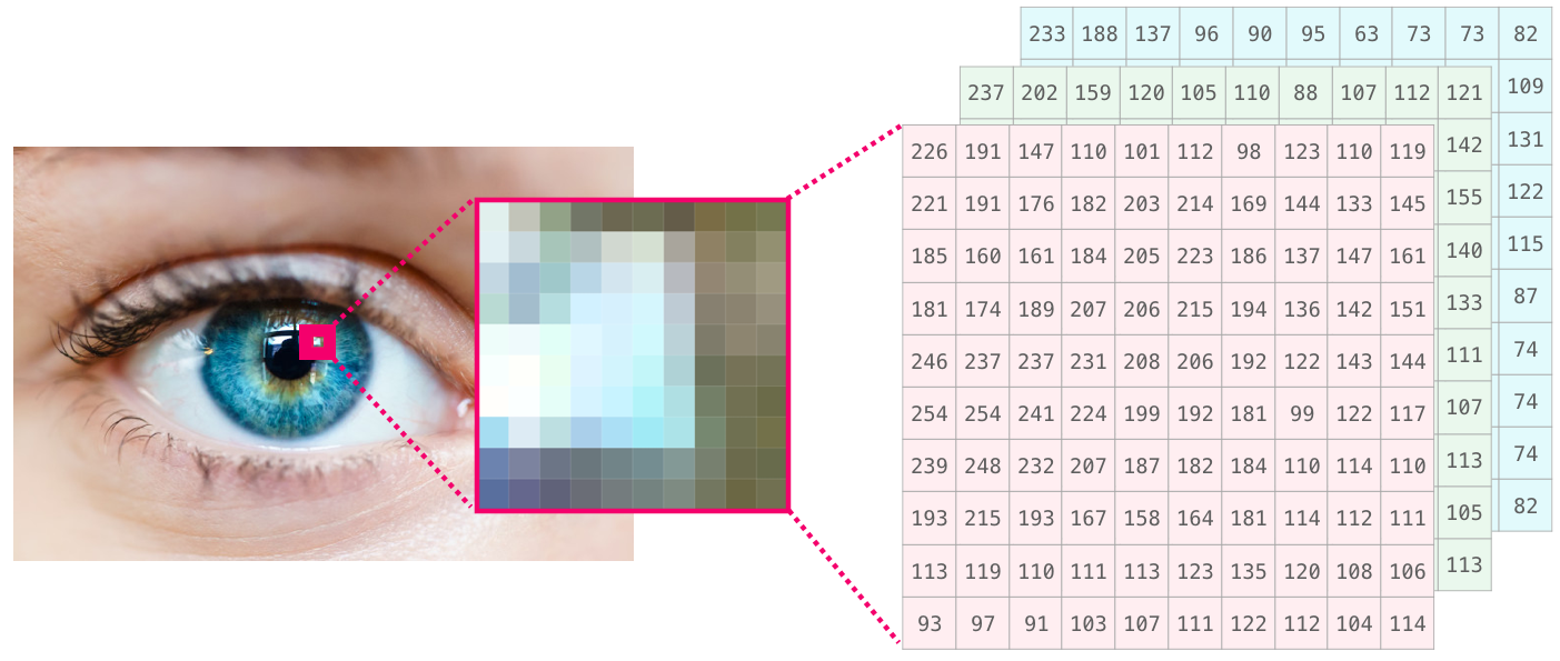
• If the image is colored, then each pixel is represented by three numbers - a value for each of red, green, and blue. In that case we need a 3rd dimension (because each cell can only contain one number). So a colored image is represented by an ndarray of dimensions: (height x width x 3).

  

Language

If we’re dealing with text, the story is a little different. The numeric representation of text requires a step of building a vocabulary (an inventory of all the unique words the model knows) and an embedding step. Let us see the steps of numerically representing this (translated) quote by an ancient spirit:

“Have the bards who preceded me left any theme unsung?”

A model needs to look at a large amount of text before it can numerically represent the anxious words of this warrior poet. We can proceed to have it process a small dataset and use it to build a vocabulary (of 71,290 words):

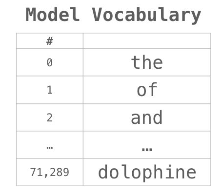
The sentence can then be broken into an array of tokens (words or parts of words based on common rules):

We then replace each word by its id in the vocabulary table:

These ids still don’t provide much information value to a model. So before feeding a sequence of words to a model, the tokens/words need to be replaced with their embeddings (50 dimension word2vec embedding in this case):

You can see that this NumPy array has the dimensions [embedding_dimension x sequence_length]. In practice these would be the other way around, but I’m presenting it this way for visual consistency. For performance reasons, deep learning models tend to preserve the first dimension for batch size (because the model can be trained faster if multiple examples are trained in parallel). This is a clear case where reshape() becomes super useful. A model like BERT, for example, would expect its inputs in the shape: [batch_size, sequence_length, embedding_size].

This is now a numeric volume that a model can crunch and do useful things with. I left the other rows empty, but they’d be filled with other examples for the model to train on (or predict).

(It turned out the poet’s words in our example were immortalized more so than those of the other poets which trigger his anxieties. Born a slave owned by his father, Antarah’s valor and command of language gained him his freedom and the mythical status of having his poem as one of seven poems suspended in the kaaba in pre-Islamic Arabia).