Houdini 中 Gray Scott Reaction-Diffusion算法的实现

这篇文章是吧很久以前学的一个神奇算法归一下档，在公交车上突然想起来了，觉得还是很有必要再仔细梳理一遍，对以后也许有用。

先看图再说话：

Gray Scott Reaction-Diffusion算法， 在模拟微观细胞的运动或者类似的效果是非常神奇。

理论链接：http://www.karlsims.com/rd.html

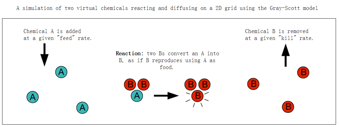
原理：模拟两种物质之间在平面（暂时是平面）上的相互作用，动作分为反应与扩散。

公式：

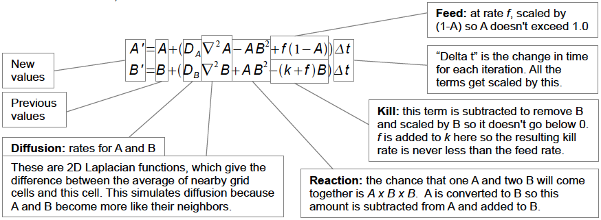
右手边第一项为扩散，第二项为反应，第三项是供给，DA与DB为分散率，▽2A或B为相邻位置扩散阵列（下图），f和k是两个非常重要的外参数，分别叫做feed和kill。可以简单理解成A是环境中的实物，两个B和一个A就能变成三个B，过程中feed会变出更多的A，k也会去掉一些B。非常想现实的生长环境。

|0.05| 0.2 |0.05|

| 0.2 | -1  | 0.2 | 

|0.05| 0.2 |0.05|    

上面是拉普拉斯方程用到的阵列，因为外围总和等于中间数的反数，所以参数化后便可以随便调

 

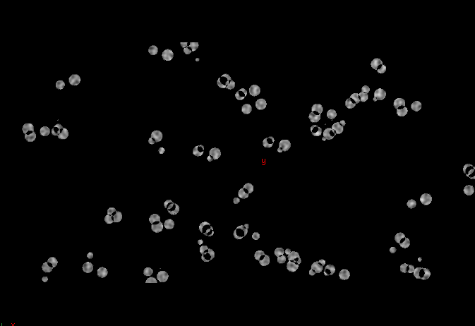
在houdini里面，使用sop solver来迭代A和B的物质变化，在进入solver前，先定义好A和B的值，一般是A在整个平面是1.0，B随机散布开，这样出来的效果也好,如下图是我做的B随机散布示意图：

同时用noise方法随机分布feed和kill的值，你当然可以使用固定的f和k，不过有随机变化的话会让生长更加自然有趣。下面是detail面板里面的简单示意：

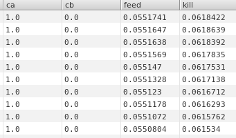
值得注意的是feed和kill的值是非常敏感的，我自己测试时，也就几个非常窄的区间内会有生长效果，要不然cb会非常快的全死掉。

在solver里面给preframe 加一个新的vex node，代码如下：

#pragma label resx "Res X"
#pragma label resy "Res Y"

#pragma label diff_a "Diffusion A"
#pragma label diff_b "Diffusion B"

#pragma label weight "Weight"
#pragma range weight 0.125 0.25

#pragma label feed "Feed"
#pragma range feed 0 1
#pragma label kill "Kill"
#pragma range kill 0 1
#pragma label time_step "Sub Step"
#pragma range time_step 0 20

#pragma hint ca invisible
#pragma hint cb invisible


//this fuction will diffuse 
float laplacian(int ptnum; int resx; int resy; string attrib; float weight){

        // | w_s  | w | w_s  |
        //-----------------------
        // | w    |-1 | w    |
        //-----------------------
        // | w_s  | w | w_s  |         weight

        // | pt+w-1  | pt+w | pt+w+1  |
        //-----------------------------
        // | pt-1    |  pt  | pt+1    |
        //-----------------------------
        // | pt-w-1  | pt-w | pt-w+1  |   location

        int vb = resx*2, hb = 1;

        // detects boundaries
        if((ptnum % resx) == 0 || (ptnum % resx) == (resx - 1)){
                hb *= -1;  // horizon
        }

        if(ptnum < resx || ptnum > (resy-1)*resx){
                vb *= -1;  // vetical
        }



        float n[];
        resize(n,9);

        float weight_second = 0.25 - weight;

        n[0] = point(0, attrib, ptnum - vb - 1) * weight_second;  // left bottom
        n[1] = point(0, attrib, ptnum - vb    ) * weight;         // bottom
        n[2] = point(0, attrib, ptnum - vb + 1) * weight_second;  // right bottom
        n[3] = point(0, attrib, ptnum      - 1) * weight;         // left
        n[4] = point(0, attrib, ptnum         ) * (-1.0);           // center
        n[5] = point(0, attrib, ptnum      + 1) * weight;         // right
        n[6] = point(0, attrib, ptnum + vb - 1) * weight_second;  // left top
        n[7] = point(0, attrib, ptnum + vb    ) * weight;         // top
        n[8] = point(0, attrib, ptnum + vb + 1) * weight_second;  // right top

        float sum=0.0;
        foreach(float i; n){
                sum += i;
        }

        return sum;
}

sop
gray_scott(
        int resx = 512;
        int resy = 512;
        float diff_a = 1.0;
        float diff_b = 1.0;
        float weight = 0.15;
        export float feed = 0.05;
        export float kill = 0.05;
        float time_step = 1.0;
        export float ca = 0.0;
        export float cb = 0.0;
        )
{
                float react_rate = ca * pow(cb,2);
                float feed_set = feed * (1.0 - ca);
                float kill_set = (kill + feed) * cb;
                //float substep = 1.0/(float)time_step;

        ca += (diff_a * laplacian(ptnum, resx, resy, "ca", weight) - react_rate + feed_set) * time_step;
        cb += (diff_b * laplacian(ptnum, resx, resy, "cb", weight) + react_rate - kill_set) * time_step;
}

 最后看一看不同的feed和kill值产生的不同效果：

 feed = 0.051  kill = 0.062

 feed = 0.0367 kill = 0.069

 feed = 0.0561 kill = 0.0636