

逻辑回归-2.逻辑回归方程及实现
逻辑回归方程
之前得出逻辑回归的损失函数:
\[J(\theta) = -\frac{1}{m}\sum_{i=1}^{m}y^{(i)}log(\sigma (X _b^{(i)} \cdot \theta))+(1-y^{(i)})log(1-\sigma (X_b^{(i)} \cdot \theta))
\]
此方程没有数学解析解,只能使用梯度下降法的方法来找到最佳的$ \theta $值,使得损失函数最小。
梯度下降法的表达式(推导过程在这里不进行阐述):
\[\frac{J(\theta)}{\theta_j} = \frac{1}{m}\sum_{i=1}^{m}(\sigma (X_b^{(i)} \cdot \theta)-y^{(i)})X_j^{(i)}
\]
比较线性回归的梯度表达式及向量化后的表达式:
\[\frac{J(\theta)}{\theta_j} = \frac{2}{m}\sum_{i=1}^{m}(X_b^{(i)} \cdot \theta-y^{(i)})X_j^{(i)}
\]
\[\Lambda J = \frac{2}{m}(X_b\theta -y)^T\cdot X_b = \frac{2}{m}X_b^T \cdot (X_b\theta -y)
\]
不难得出逻辑回归向量化后的梯度表达式:
\[\Lambda J = \frac{1}{m}X_b^T \cdot (\sigma (X_b\theta) -y)
\]
算法实现
加载鸢尾花数据集
import numpy
from sklearn import datasets
from mylib import LogisticRegression
from matplotlib import pyplot

iris = datasets.load_iris()
X = iris.data
y = iris.target

# 取y值为0和1的数据,为了数据可视化,特征只取两个
X = X[y<2,:2]
y = y[y<2]
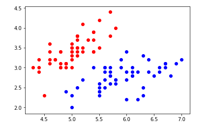
绘制数据集
pyplot.scatter(X[y==0,0],X[y==0,1],color='red')
pyplot.scatter(X[y==1,0],X[y==1,1],color='blue')
pyplot.show()
用封装好的逻辑回归,查看准确率:
from mylib.model_selection import train_test_split

x_train,x_test,y_train,y_test = train_test_split(X,y,seed =666)

logic_reg = LogisticRegression.LogisticRegression()
logic_reg.fit(x_train,y_train)
logic_reg.score(x_test,y_test)
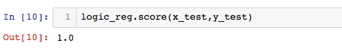
可以看出,预测准确率100%
