梯度下降法-1.原理及简单实现

梯度下降法 （Gradient Descent）

• 不是一个机器学习算法
• 是一种基于搜索的最优化方法
• 作用：最小化一个损失函数 （梯度上升法：最大化一个效用函数）

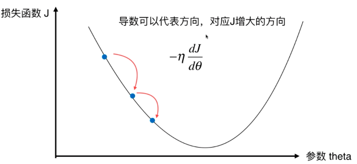
原理 - 寻找损失函数J的最小值

\[\frac{dJ}{d\theta} = \frac{J_{\theta +1}-J_\theta }{\Delta \theta } \]

导数代表theta单位变化时，J相应的变化,导数也可以代表方向，对应J增大的方向

\[\theta = \theta -\eta \frac{dJ}{d\theta} \]

$\eta $ 为移动步长，关于$\eta $：

• $\eta $ 称为学习率
• $\eta $ 的取值影响获得最优解的速度
• $\eta $ 取值不合适，甚至得不到最优解
• $\eta $ 是梯度下降法中的一个超参数

注意，如下图所示,不是所有的函数都有唯一的极致点

解决办法：多次运行，随机化初始点（初始点也是梯度下降法的一个超参数）

模拟实现梯度下降法

import numpy
import matplotlib.pyplot as plt

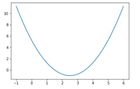
#从-1到6之间，取140个点
plot_x = numpy.linspace(-1,6, 140) 
# 绘制一个二次函数
plot_y = (plot_x - 2.5)**2-1 

plt.plot(plot_x,plot_y)
plt.show() 

J函数表达式

 def J(theta):
    try:
        return (theta-2.5)**2-1
    except:
        return float('inf')  #避免J太大

J函数的导数

def dJ(theta):
    return 2*(theta-2.5) 

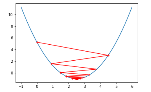
梯度下降法核心

# 初始点
theta = 0.0  
# 梯度下降的学习率
eta =0.1
espilon = 1e-8   #代表一个接近于0的数
theta_history = [theta]
while True:
    gradient = dJ(theta)   #导数代表了切线斜率
    last_theta = theta
    theta = theta - eta * gradient
    theta_history.append(theta)
    if abs(theta - last_theta) < espilon:
        break
print(theta,J(theta),dJ(theta))
plt.plot(plot_x,J(plot_x))
plt.plot(numpy.array(theta_history),J(numpy.array(theta_history)),color='r', marker='+')
plt.show()

增大学习率 $\eta $
eta = 0.9时：

eta = 1.1时：

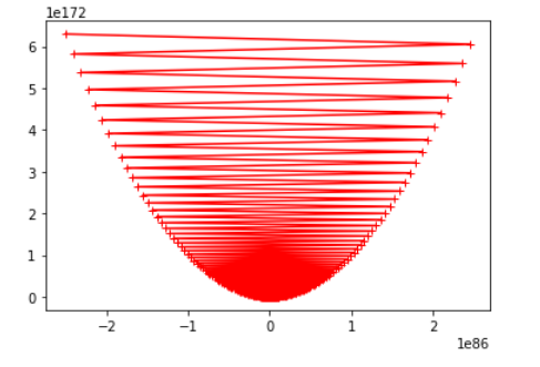
由上图可看出，随着步长 $\eta $ 选取的愈来愈大，梯度下降的过程开始变得不收敛