机器学习 - 案例 - 集成算法 - 泰坦尼克船员获救 (特征分析, 数据预处理, 线性, 逻辑, 随机, 调参, 特征衡量, 集成)
样本数据
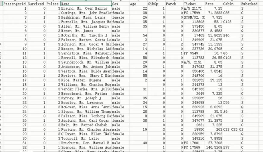
PassengerId,Survived,Pclass,Name,Sex,Age,SibSp,Parch,Ticket,Fare,Cabin,Embarked
1,0,3,"Braund, Mr. Owen Harris",male,22,1,0,A/5 21171,7.25,,S
2,1,1,"Cumings, Mrs. John Bradley (Florence Briggs Thayer)",female,38,1,0,PC 17599,71.2833,C85,C
3,1,3,"Heikkinen, Miss. Laina",female,26,0,0,STON/O2. 3101282,7.925,,S
4,1,1,"Futrelle, Mrs. Jacques Heath (Lily May Peel)",female,35,1,0,113803,53.1,C123,S
5,0,3,"Allen, Mr. William Henry",male,35,0,0,373450,8.05,,S
6,0,3,"Moran, Mr. James",male,,0,0,330877,8.4583,,Q
7,0,1,"McCarthy, Mr. Timothy J",male,54,0,0,17463,51.8625,E46,S
8,0,3,"Palsson, Master. Gosta Leonard",male,2,3,1,349909,21.075,,S
9,1,3,"Johnson, Mrs. Oscar W (Elisabeth Vilhelmina Berg)",female,27,0,2,347742,11.1333,,S
10,1,2,"Nasser, Mrs. Nicholas (Adele Achem)",female,14,1,0,237736,30.0708,,C
11,1,3,"Sandstrom, Miss. Marguerite Rut",female,4,1,1,PP 9549,16.7,G6,S
12,1,1,"Bonnell, Miss. Elizabeth",female,58,0,0,113783,26.55,C103,S
13,0,3,"Saundercock, Mr. William Henry",male,20,0,0,A/5. 2151,8.05,,S
14,0,3,"Andersson, Mr. Anders Johan",male,39,1,5,347082,31.275,,S
15,0,3,"Vestrom, Miss. Hulda Amanda Adolfina",female,14,0,0,350406,7.8542,,S
16,1,2,"Hewlett, Mrs. (Mary D Kingcome) ",female,55,0,0,248706,16,,S
17,0,3,"Rice, Master. Eugene",male,2,4,1,382652,29.125,,Q
18,1,2,"Williams, Mr. Charles Eugene",male,,0,0,244373,13,,S
特征数据分析
脑测
PassengerId 编号, 没啥意义
Survived 是否获救 (预测结果)
Pclass 船舱等级 -- > 等级越好越大?
Name 姓名 -- > 名字越长越大? 玄学 (贵族名字长? 获救几率大?)
Sex 性别 -- > 女性更大几率?
Age 年龄 -- > 青壮年更大几率?
SibSp 兄弟姐妹数量 -- > 亲人越多越大 ?
Parch 老人孩子数量 -- > 越多越小?
Ticket 票编号 -- > 越大越高? 玄学 (票头排列和船舱有关也有可能?)
Fare 票价 -- > 越贵越大?
Cabin 住舱编号 -- > 这列数据缺失值很多, 以及表达意义..? (可能靠近夹板位置容易获救?)
Embarked 上站点 -- > 不同的站点的人体格不一样? 运气不一样? 玄学
数据分析
以上都是简单的人为猜测, 用 py代码进行所有特征数据的详细数学统计信息展示
总数 / 平均值 / 标准差 / 最小 / 四分之一数 / 众数 / 四分之三数 / 最大值
代码
import pandas #ipython notebook
titanic = pandas.read_csv("titanic_train.csv")
# titanic.head(5)
print (titanic.describe())
       PassengerId    Survived      Pclass         Age       SibSp  \
count   891.000000  891.000000  891.000000  714.000000  891.000000
mean    446.000000    0.383838    2.308642   29.699118    0.523008
std     257.353842    0.486592    0.836071   14.526497    1.102743
min       1.000000    0.000000    1.000000    0.420000    0.000000
25%     223.500000    0.000000    2.000000   20.125000    0.000000
50%     446.000000    0.000000    3.000000   28.000000    0.000000
75%     668.500000    1.000000    3.000000   38.000000    1.000000
max     891.000000    1.000000    3.000000   80.000000    8.000000

            Parch        Fare
count  891.000000  891.000000
mean     0.381594   32.204208
std      0.806057   49.693429
min      0.000000    0.000000
25%      0.000000    7.910400
50%      0.000000   14.454200
75%      0.000000   31.000000
max      6.000000  512.329200
数据预处理
缺失填充
分析
总数据行数为 891 行, 而 age 只有 714 行存在数据缺失
age 的指标在我们的人为分析中是较为重要的指标, 因此不能忽略的
需要进行缺失数据的填充
代码
这里使用均值进行填充
函数方法 .fillna() 为空数据填充 , 参数为填充数据
.median() 为平均值计算
titanic["Age"] = titanic["Age"].fillna(titanic["Age"].median())
print (titanic.describe())
       PassengerId    Survived      Pclass         Age       SibSp  \
count   891.000000  891.000000  891.000000  891.000000  891.000000
mean    446.000000    0.383838    2.308642   29.361582    0.523008
std     257.353842    0.486592    0.836071   13.019697    1.102743
min       1.000000    0.000000    1.000000    0.420000    0.000000
25%     223.500000    0.000000    2.000000   22.000000    0.000000
50%     446.000000    0.000000    3.000000   28.000000    0.000000
75%     668.500000    1.000000    3.000000   35.000000    1.000000
max     891.000000    1.000000    3.000000   80.000000    8.000000

            Parch        Fare
count  891.000000  891.000000
mean     0.381594   32.204208
std      0.806057   49.693429
min      0.000000    0.000000
25%      0.000000    7.910400
50%      0.000000   14.454200
75%      0.000000   31.000000
max      6.000000  512.329200
字符串转化数组处理
分析
性别这里的数据填充为 ['male' 'female']
这里出现的可能性只有两种, Py对非数值得数据进行数据分析兼容性很不友好
这里需要转换成数字更容易处理, 同理此分析适用于 Embarked 也是相同的处理方式
但是 Embarked 还存在缺失值的问题, 这里就没办法用均值了, 但是可以使用众数, 即最多的来填充
代码
print titanic["Sex"].unique() # ['male' 'female']

# Replace all the occurences of male with the number 0.
titanic.loc[titanic["Sex"] == "male", "Sex"] = 0
titanic.loc[titanic["Sex"] == "female", "Sex"] = 1
print( titanic["Embarked"].unique()) # ['S' 'C' 'Q' nan]
titanic["Embarked"] = titanic["Embarked"].fillna('S')
titanic.loc[titanic["Embarked"] == "S", "Embarked"] = 0
titanic.loc[titanic["Embarked"] == "C", "Embarked"] = 1
titanic.loc[titanic["Embarked"] == "Q", "Embarked"] = 2
线性回归
一上来还是用最简单的方式线性回归来实现预测模型
模块
线性回归模块 LinearRegression 以及数据集划分交叉验证的模块 KFold
from sklearn.linear_model import LinearRegression
from sklearn.model_selection import KFold
代码
线性回归 / 交叉验证
from sklearn.linear_model import LinearRegression
from sklearn.model_selection import KFold

# 预备选择的特征
predictors = ["Pclass", "Sex", "Age", "SibSp", "Parch", "Fare", "Embarked"]

# 线性回归模型实例化
alg = LinearRegression()
# 交叉验证实例化, 划分三份, 随机打乱种子为 0
kf = KFold(n_splits=3, shuffle=False, random_state=0)

predictions = []

# 交叉验证划分训练集测试集, 对每一份进行循环
for train, test in kf.split(titanic):
    # 拿到训练数据 (仅特征值列)
    train_predictors = (titanic[predictors].iloc[train,:])
    # 拿到训练数据的目标 (仅目标值列)
    train_target = titanic["Survived"].iloc[train]
    # 训练线性回归
    alg.fit(train_predictors, train_target)
    # 在测试集上进行预测
    test_predictions = alg.predict(titanic[predictors].iloc[test,:])
    predictions.append(test_predictions)
计算准确率
最后得出的结果其实就是是否获救的二分类问题, 按照分类是否大于 0.5进行判定
import numpy as np

predictions = np.concatenate(predictions, axis=0)

predictions[predictions > .5] = 1
predictions[predictions <=.5] = 0
accuracy = sum(predictions==titanic['Survived'])/len(predictions)
print(accuracy)  # 0.7833894500561167
最终结果为 0.78 不算高
逻辑回归
对于想要一个概率值得情况可以使用逻辑回归
from sklearn.model_selection import cross_val_score
from sklearn.linear_model import LogisticRegression

# 实例化, 指定 solver 避免警告提示
alg = LogisticRegression(solver="liblinear",random_state=1)

scores = cross_val_score(alg, titanic[predictors], titanic["Survived"], cv=3)

print(scores.mean())
0.7878787878787877
逻辑回归的结果也差不多少
随机森林
对于一个新的模型的建立和预测选择分类器的时候, 一上来还是更推荐使用随机森林
随机森林大概率会比其他的结果要好一点
模块
from sklearn.model_selection import cross_val_score
from sklearn.model_selection import KFold
from sklearn.ensemble import RandomForestClassifier
构造随机森林 / 交叉验证
from sklearn.model_selection import cross_val_score
from sklearn.model_selection import KFold
from sklearn.ensemble import RandomForestClassifier

predictors = ["Pclass", "Sex", "Age", "SibSp", "Parch", "Fare", "Embarked"]

# n_estimators 构造多少树
# min_samples_split 最小切分数量
# min_samples_leaf 最少叶子节点个数
# tree branch(分支) ends (the bottom points of the tree)
alg = RandomForestClassifier(random_state=1,
                             n_estimators=10,
                             min_samples_split=2,
                             min_samples_leaf=1)

# 交叉验证
kf = KFold(n_splits=3, shuffle=False, random_state=1)
scores = cross_val_score(alg, titanic[predictors], titanic["Survived"], cv=kf)

# 得出的准确率分值平均一下
print(scores.mean()) # 0.7856341189674523
由此得出的结果也不怎么理想, 在进行参数调优处理
随机森林参数调优
对构建随机森林的参数进行调优, 可以让准确率达到 81
# 调整最大构建树的数量从 10 到 100
# 为了防止树高度过高, 调整最小切分从 2 到 4
# 为了防止树高度过高, 调整最少叶子从 1 到 2

alg = RandomForestClassifier(random_state=1,
                             n_estimators=50,
                             min_samples_split=4,
                             min_samples_leaf=2)

kf = KFold(n_splits=3, shuffle=False, random_state=1)
scores = cross_val_score(alg, titanic[predictors], titanic["Survived"], cv=kf)


print(scores.mean())  # 0.8159371492704826
在参数调优之后, 模型的这块已经没办法再继续提升了
就要想办法在别的地方再看看有什么好办法来提升, 这时需要回归数据
特征调优
特征分析
# 预备选择的特征
predictors = ["Pclass", "Sex", "Age", "SibSp", "Parch", "Fare", "Embarked"]
在此之前使用的特征就是以上这些, 有些特征还是没利用上的
黔驴技穷的情况下我们这些潜在的之前觉得没有用的特征就要再加上了
特征添加
这里多加一个特征
FamilySize 表示亲人数量, 是兄弟姐妹数量和老人孩子数量的价格 处于的考虑是人多力量大..?
再多加一个特征
NameLength 表示名字长度, 基于的考量是名字越长可能是贵族容易获救...? 或者只是单纯的玄学
titanic["FamilySize"] = titanic["SibSp"] + titanic["Parch"]
titanic["NameLength"] = titanic["Name"].apply(lambda x: len(x))
在处理名字的时候我们发现外国人的名字喜欢加上很多的称呼, Mr 男士, Miss 女士, Master,Dr 之类的
这些的称呼或者头衔代表的了某些性质可能也会影响到最终结果是否获救, 在这里在进行一次提取
对这些称呼建立映射新加一个 特征 Title 表示头衔
import re

# 提取 title 函数
def get_title(name):
    title_search = re.search(' ([A-Za-z]+)\.', name)
    if title_search:
        return title_search.group(1)
    return ""

# 对每行数据的 Name 遍历执行 get_title 函数
titles = titanic["Name"].apply(get_title)
print(pandas.value_counts(titles))

title_mapping = {
    "Mr": 1,
    "Miss": 2,
    "Mrs": 3,
    "Master": 4,
    "Dr": 5,
    "Rev": 6,
    "Major": 7,
    "Col": 7,
    "Mlle": 8,
    "Mme": 8,
    "Don": 9,
    "Lady": 10,
    "Countess": 10,
    "Jonkheer": 10,
    "Sir": 9,
    "Capt": 7,
    "Ms": 2
}
for k, v in title_mapping.items():
    titles[titles == k] = v

# 验证我们是否转换了所有内容
print(pandas.value_counts(titles))

# 加入到样本数据中
titanic["Title"] = titles
打印结果, 可见前三个占比是绝大多数
Mr          517
Miss        182
Mrs         125
Master       40
Dr            7
Rev           6
Col           2
Major         2
Mlle          2
Countess      1
Ms            1
Lady          1
Jonkheer      1
Don           1
Mme           1
Capt          1
Sir           1
Name: Name, dtype: int64
1     517
2     183
3     125
4      40
5       7
6       6
7       5
10      3
8       3
9       2
Name: Name, dtype: int64
特征重要性分析
原理
12345 特征建立随机森林后计算得出错误率 为 x
将 3 特征的数据进行噪音化处理使其成为脏数据 假设为 '3'
再次计算 12'3'45 的的模型计算错误率为 y
x 和 y 之前的差值越大表示 3 特征对模型的影响越大, 反正则越小
代码
import numpy as np
from sklearn.feature_selection import SelectKBest, f_classif # 选择最好特征
import matplotlib.pyplot as plt

# 所有特征列表
predictors = [
    "Pclass", "Sex", "Age", "SibSp", "Parch", "Fare", "Embarked", "FamilySize",
    "Title", "NameLength"
]


# 执行特征选择
selector = SelectKBest(f_classif, k=5)
selector.fit(titanic[predictors], titanic["Survived"])

scores = -np.log10(selector.pvalues_)

plt.bar(range(len(predictors)), scores)
plt.xticks(range(len(predictors)), predictors, rotation='vertical')
plt.show()

# 只选择4个最好的特征
predictors = ["Pclass", "Sex", "Fare", "Title"]

alg = RandomForestClassifier(random_state=1,
                             n_estimators=50,
                             min_samples_split=8,
                             min_samples_leaf=4)
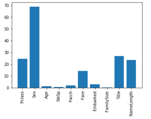
分析
由此可见和之前的脑测分析存在不小的差距, 年龄家庭并没有很大的影响
船票价格可能和船舱等级有关, 因此都有较大影响
最大的影响还是性别, 女性在这方面享有了生命优先的权益
有趣的是名字前缀和名字长度也存在不小的关系
集成算法
在不考虑时空复杂度的情况下单一的为了追求结果, 我们这里在使用集成算法
注意使用集成算法的时候被集成的算法最好使用远离不同的算法进行集成从而更多方面的对数据进行建模从而取均值
原理
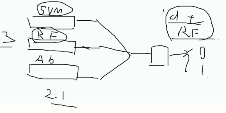
比如图中使用了 SVM , RF , AB 三个算法进行集成
尽量不要使用相同类似原理的算法进行集成, 比如 DT, RF 一起
对某一数据的结果进行预测的时候 以少数服从多数的原则决定最终的结果
这样得出的结果会考虑更多元性因此也更加精准
代码
from sklearn.ensemble import GradientBoostingClassifier
import numpy as np

# The algorithms we want to ensemble.
# We're using the more linear predictors for the logistic regression, and everything with the gradient boosting classifier.
algorithms = [
    [GradientBoostingClassifier(random_state=1, n_estimators=25, max_depth=3), ["Pclass", "Sex", "Age", "Fare", "Embarked", "FamilySize", "Title",]],
    [LogisticRegression(random_state=1,solver='liblinear'), ["Pclass", "Sex", "Fare", "FamilySize", "Title", "Age", "Embarked"]]
]

# 交叉验证
kf = KFold(n_splits=3,shuffle=False, random_state=1)

predictions = []
for train, test in kf.split(titanic):
    train_target = titanic["Survived"].iloc[train]
    full_test_predictions = []
    # 对每一个算法进行训练预测
    for alg, predictors in algorithms:
        # 训练数据模型
        alg.fit(titanic[predictors].iloc[train,:], train_target)
        # 预测
        # The .astype(float) is necessary to convert the dataframe to all floats and avoid an sklearn error.
        test_predictions = alg.predict_proba(titanic[predictors].iloc[test,:].astype(float))[:,1]
        full_test_predictions.append(test_predictions)
    # 最终的结果是对两个分类器的结果取平均处理从而判断是否得救
    test_predictions = (full_test_predictions[0] + full_test_predictions[1]) / 2
    # 对是否得救进行 0 1 处理
    test_predictions[test_predictions <= .5] = 0
    test_predictions[test_predictions > .5] = 1
    predictions.append(test_predictions)

# 将所有的预测放在一个数组中
predictions = np.concatenate(predictions, axis=0)

# 计算准确率
accuracy = sum(predictions == titanic["Survived"]) / len(predictions)
print(accuracy)
0.8215488215488216
最终的结果为 0.82 上升了一丢丢
实际结果预测
对以上的模型准确率结果进行一个简单的对比吧
线性 0.7833894500561167
逻辑 0.7878787878787877
随机 0.7856341189674523
调机 0.8159371492704826
集成 0.8215488215488216
最终使用集成算法的模型预测测试集试下
代码
预处理
对测试集还是要做个预处理, 新佳乐title 的特征, 因为上面的分析中这个的特征还是不能忽略的
titles = titanic_test["Name"].apply(get_title)

title_mapping = {
    "Mr": 1,
    "Miss": 2,
    "Mrs": 3,
    "Master": 4,
    "Dr": 5,
    "Rev": 6,
    "Major": 7,
    "Col": 7,
    "Mlle": 8,
    "Mme": 8,
    "Don": 9,
    "Lady": 10,
    "Countess": 10,
    "Jonkheer": 10,
    "Sir": 9,
    "Capt": 7,
    "Ms": 2,
    "Dona": 10
}
for k, v in title_mapping.items():
    titles[titles == k] = v
titanic_test["Title"] = titles

print(pandas.value_counts(titanic_test["Title"]))

titanic_test["FamilySize"] = titanic_test["SibSp"] + titanic_test["Parch"]
1     240
2      79
3      72
4      21
7       2
6       2
10      1
5       1
Name: Title, dtype: int64
预测结果
predictors = [
    "Pclass", "Sex", "Age", "Fare", "Embarked", "FamilySize", "Title"
]

algorithms = [
    [
        GradientBoostingClassifier(random_state=1,
                                   n_estimators=25,
                                   max_depth=3), predictors
    ],
    [
        LogisticRegression(random_state=1, solver='liblinear'),
        ["Pclass", "Sex", "Fare", "FamilySize", "Title", "Age", "Embarked"]
    ]
]

full_predictions = []
for alg, predictors in algorithms:

    alg.fit(titanic[predictors], titanic["Survived"])

    predictions = alg.predict_proba(
        titanic_test[predictors].astype(float))[:, 1]
    predictions[predictions <= .5] = 0
    predictions[predictions > .5] = 1
    full_predictions.append(predictions)


# predictions = (full_predictions[0] * 3 + full_predictions[1]) / 4
predictions
array([0., 0., 0., 0., 1., 0., 1., 0., 1., 0., 0., 0., 1., 0., 1., 1., 0.,
       0., 1., 1., 0., 0., 1., 0., 1., 0., 1., 0., 0., 0., 0., 0., 0., 1.,
       0., 0., 1., 1., 0., 0., 0., 0., 0., 1., 1., 0., 0., 0., 1., 0., 0.,
       0., 1., 1., 0., 0., 0., 0., 0., 1., 0., 0., 0., 1., 1., 1., 1., 0.,
       0., 1., 1., 0., 1., 0., 1., 1., 0., 1., 0., 1., 0., 0., 0., 0., 0.,
       0., 1., 1., 1., 1., 1., 0., 1., 0., 0., 0., 1., 0., 1., 0., 1., 0.,
       0., 0., 1., 0., 0., 0., 0., 0., 0., 1., 1., 1., 1., 0., 0., 1., 0.,
       1., 1., 0., 1., 0., 0., 1., 0., 1., 0., 0., 0., 1., 0., 0., 0., 0.,
       0., 0., 1., 0., 0., 1., 0., 0., 0., 0., 0., 0., 0., 0., 1., 0., 0.,
       0., 0., 0., 1., 1., 0., 1., 1., 0., 1., 0., 0., 1., 0., 0., 1., 1.,
       0., 0., 0., 0., 0., 1., 1., 0., 1., 1., 0., 0., 1., 0., 1., 0., 1.,
       0., 0., 0., 0., 0., 0., 0., 0., 0., 1., 1., 0., 1., 1., 0., 1., 1.,
       0., 0., 1., 0., 1., 0., 0., 0., 0., 1., 0., 0., 1., 0., 1., 0., 1.,
       0., 1., 0., 1., 1., 0., 1., 0., 0., 0., 1., 0., 0., 0., 0., 0., 0.,
       1., 1., 1., 1., 0., 0., 0., 0., 1., 0., 1., 1., 1., 0., 1., 0., 0.,
       0., 0., 0., 1., 0., 0., 0., 1., 1., 0., 0., 0., 0., 1., 0., 0., 0.,
       1., 1., 0., 1., 0., 0., 0., 0., 1., 0., 1., 1., 1., 0., 0., 0., 0.,
       0., 0., 1., 0., 0., 0., 0., 1., 0., 0., 0., 0., 0., 0., 0., 1., 1.,
       0., 0., 0., 0., 0., 0., 0., 1., 1., 1., 0., 0., 0., 0., 0., 0., 0.,
       0., 1., 0., 1., 0., 0., 0., 1., 0., 0., 1., 0., 0., 0., 0., 0., 0.,
       0., 0., 0., 1., 0., 1., 0., 1., 0., 1., 1., 0., 0., 0., 1., 0., 1.,
       0., 0., 1., 0., 1., 1., 0., 1., 0., 0., 1., 1., 0., 0., 1., 0., 0.,
       1., 1., 1., 0., 0., 0., 0., 0., 1., 1., 0., 1., 0., 0., 0., 0., 1.,
       1., 0., 0., 0., 1., 0., 1., 0., 0., 1., 0., 1., 1., 0., 0., 0., 0.,
       1., 1., 1., 1., 1., 0., 1., 0., 0., 0.])
总结
数据分析 - 已有特征分析, 提取另加特征
预处理 - 缺失值的处理, 字符数据映射
算法 - 多种算法的尝试比对, 模型参数调优
特征重要性 - 特征重要性的比对, 去除无用特征等
集成 - 集成算法作为最后的手段
本文来自博客园,作者:羊驼之歌,转载请注明原文链接:https://www.cnblogs.com/shijieli/p/11806993.html