A/B Testing with Practice in Python (Part One)
I learned A/B testing from a Youtube vedio. The link is https://www.youtube.com/watch?v=Bu7OqjYk0jM.
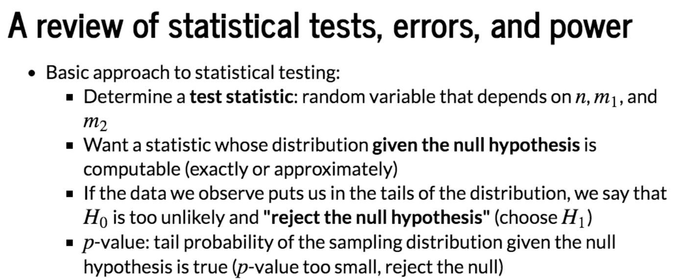
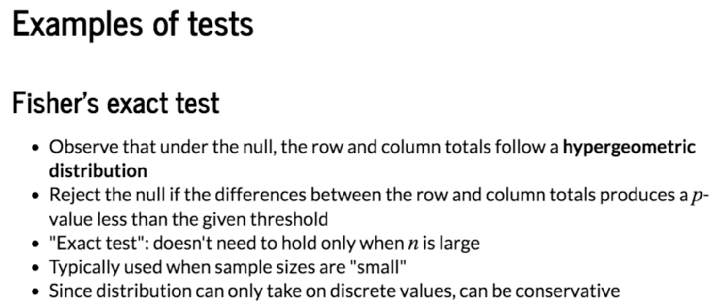
I will divide the note into two parts. The first part is generally an overview of hypothesis testing. Most concepts can be found in the article "Statistics Basics: Main Concepts in Hypothesis Testing" and I will focus on pratical applications here.



|
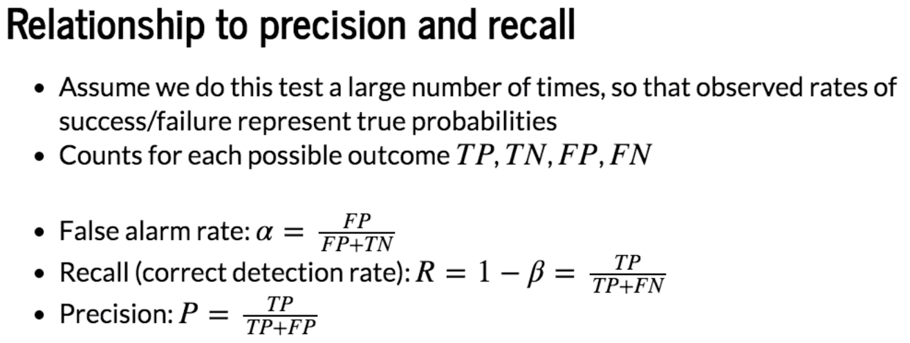
Actual Predicted |
T (H1) | F (H0) |
| T (H1) | TP | FP (α) |
| F (H0) | FN (β) | TN |
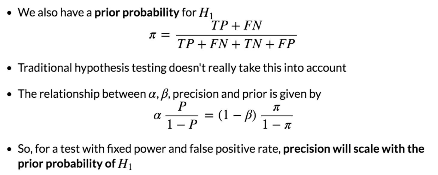
P = TP/(TP+FN)
R = 1-β =TP/(TP+FN)

Python Example
Case #1: Alternate hypothesis is true
n = 100
p1 = 0.4
p2 = 0.6

# Compute distributions
x = np.arange(0,n+1)
pmf1 = stats.binom.pmf(x,n,p1)
pmf2 = stats.binom.pmf(x,n,p2)
plot(x,pmf1,pmf2)

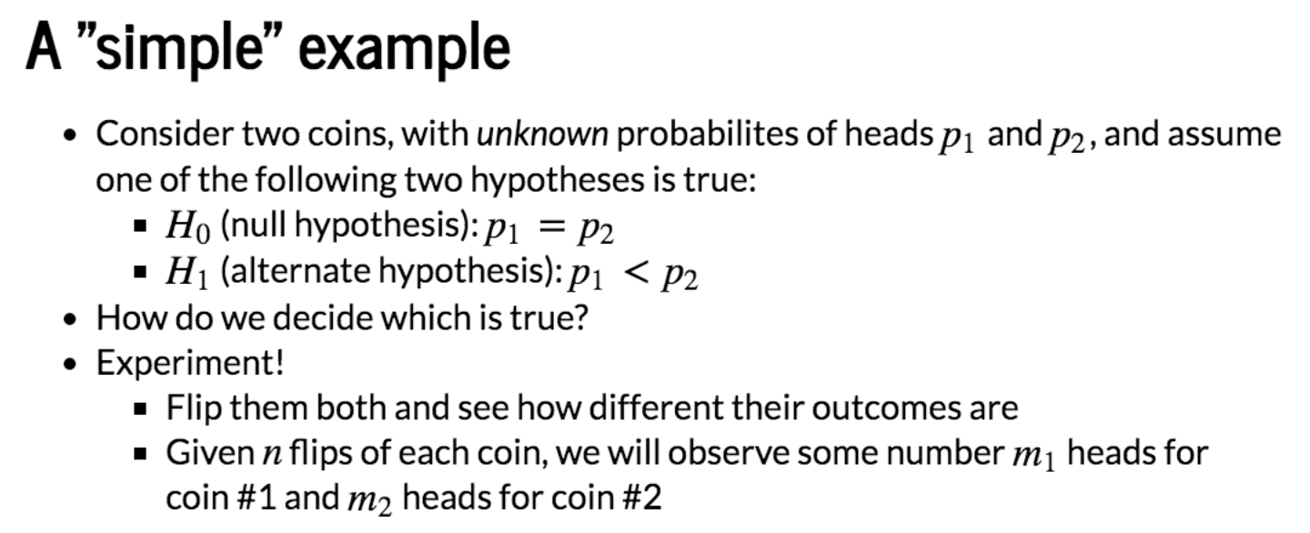
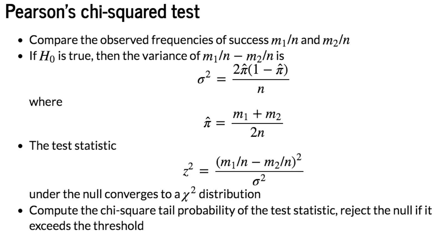
We can find that the distributions between Coin 1 and Coin 2 are different. We check different values of m1 and m2.
# Example outcomes
m1, m2 = 40, 60
table = [[m1, n-m1], [m2, n-m2]]
chi2, pval, dof, expected = stats.chi2_contingency(table)
decision = 'reject H0' if pval<0.05 else 'accept H0'
print('{} ({})'.format(pval,decision))
0.007209570764742524 (reject H0)
# Example outcomes
m1, m2 = 43, 57
table = [[m1, n-m1], [m2, n-m2]]
chi2, pval, dof, expected = stats.chi2_contingency(table)
decision = 'reject H0' if pval<0.05 else 'accept H0'
print('{} ({})'.format(pval,decision))
0.06599205505934735 (accept H0)
In the secod example, m1 and m2 are not different significantly to reject H0.
Case #2: Null hypothesis is true
n = 100
p1 = 0.5
p2 = 0.5

# Compute distributions
x = np.arange(0,n+1)
pmf1 = stats.binom.pmf(x,n,p1)
pmf2 = stats.binom.pmf(x,n,p2)
plot(x,pmf1,pmf2)

In this case, two distributions overlap because we define the same value of p1 and p2.
# Example outcomes
m1, m2 = 49, 51
table = [[m1, n-m1], [m2, n-m2]]
chi2, pval, dof, expected = stats.chi2_contingency(table)
decision = 'reject H0' if pval<0.05 else 'accept H0'
print('{} ({})'.format(pval,decision))
0.887537083981715 (accept H0)
Actuall, we can only say that m1 and m2 are not different significantly to reject H0. It doesn't mean we should accept H0. The explanation is given in the previous article.
# Example outcomes
m1, m2 = 42, 58
table = [[m1, n-m1], [m2, n-m2]]
chi2, pval, dof, expected = stats.chi2_contingency(table)
decision = 'reject H0' if pval<0.05 else 'accept H0'
print('{} ({})'.format(pval,decision))


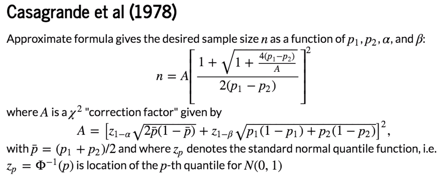

Firstly, calculate the sample size:
p1, p2 = 0.0500, 0.0515
alpha = 0.05
beta = 0.05

# Evaluate quantile function
p_bar = (p1+p2)/2.0
za = stats.norm.ppf(1-alpha/2) # Two-sided test
zb = stats.norm.ppf(1-beta)

# Compute correction factor
A = (za*np.sqrt(2*p_bar*(1-p_bar))+ zb*np.sqrt(p1*(1-p1)+p2*(1-p2)))**2

#Estimate samples required
n = A*(((1+np.sqrt(1+4*(p1-p2)/A)))/(2*(p1-p2)))**2

print (n) # we need 2n users
So for test and control combined we'll need at least 2n = 1.1 million users. This is where this stuff gets hard and you're trying to measure something that doesn't happen often which is usally the thing to care because if it's rare, it's usually valuable. When you're trying to change it, you usually can't change it much because if you can change it a lot then your business would be easier usually it's harder to change the thing you care the most about. So in that case, it's like the hardest case where a/b testing the most values are unchange.
Next we can perform a/b testing:
n = 555119
n_trials = 10000

# Simulate experimental results when null is true
control0 = stats.binom.rvs (n,p1,size = n_trials)
test0 = stats.binom.rvs(n, p1, size = n_trials) # Test and control are the same
tables0 = [[[a, n-a], [b, n-b]] for a, b in zip(control0, test0)]
results0 = [stats.chi2_contingency(T) for T in tables0]
decisions0 = [x[1] <= alpha for x in results0]

# Simulate experimental results when alternate is true
control1 = stats.binom.rvs (n,p1,size = n_trials)
test1 = stats.binom.rvs(n, p2, size = n_trials) # Test and control are the same
tables1 = [[[a, n-a], [b, n-b]] for a, b in zip(control1, test1)]
results1 = [stats.chi2_contingency(T) for T in tables1]
decisions1 = [x[1] <= alpha for x in results1]

# Compute false alarm and correct detection rates
alpha_est = sum(decisions0)/float(n_trials)
power_est = sum(decisions1)/float(n_trials)

print('Theoretical false alarm rate = {:0.4f}, '.format(alpha)+
     'empirical false alarm rate = {:0.4f}'.format(alpha_est))
print('Theoretical power = {:0.4f}, '.format(1-beta)+
     'empirical power = {:0.4f}'.format(power_est))
Theoretical false alarm rate = 0.0500, empirical false alarm rate = 0.0509
Theoretical power = 0.9500, empirical power = 0.9536


 浙公网安备 33010602011771号