用R来分析洛杉矶犯罪

由于微信不允许外部链接，你需要点击文章尾部左下角的 "阅读原文"，才能访问文中链接。

洛杉矶市（Los Angeles）或”爵士乐的诞生地（The Birthplace of Jazz）”是美利坚合众国人口最多的城市之一，人口估计超过四百万。 在这样规模的城市，它的犯罪率是值得我们去探索的。

本项目旨在探讨 2017 年度的犯罪率。这个项目中使用的数据集是在洛杉矶警察局提供的这个链接中下载的（参考文章末尾小编提供的该完整 CSV 数据下载，约 400 M）。

数据准备

library(data.table) #faster way to read large dataset
library(tidyverse) #load dplyr, tidyr and ggplot
library(ggmap) #use to read map
library(maps) #map tools kits
library(mapdata) #read the map data
library(lubridate) #date manuplation
library(ggrepel) #better label
library(varhandle) #load the function unfactor

crime_la <- as.data.frame(fread("Crime_Data_from_2010_to_Present.csv", na.strings = c("NA")))
glimpse(crime_la)

Read 1810088 rows and 26 (of 26) columns from 0.390 GB file in 00:00:05
Observations: 1,810,088
Variables: 26
$ `DR Number`              <int> 1208575, 102005556, 418, 101822289, 421044...
$ `Date Reported`          <chr> "03/14/2013", "01/25/2010", "03/19/2013", ...
$ `Date Occurred`          <chr> "03/11/2013", "01/22/2010", "03/18/2013", ...
$ `Time Occurred`          <int> 1800, 2300, 2030, 1800, 2300, 1400, 2230, ...
$ `Area ID`                <int> 12, 20, 18, 18, 21, 1, 11, 16, 19, 9, 19, ...
$ `Area Name`              <chr> "77th Street", "Olympic", "Southeast", "So...
$ `Reporting District`     <int> 1241, 2071, 1823, 1803, 2133, 111, 1125, 1...
$ `Crime Code`             <int> 626, 510, 510, 510, 745, 110, 510, 510, 51...
$ `Crime Code Description` <chr> "INTIMATE PARTNER - SIMPLE ASSAULT", "VEHI...
$ `MO Codes`               <chr> "0416 0446 1243 2000", "", "", "", "0329",...
$ `Victim Age`             <int> 30, NA, 12, NA, 84, 49, NA, NA, NA, 27, NA...
$ `Victim Sex`             <chr> "F", "", "", "", "M", "F", "", "", "", "F"...
$ `Victim Descent`         <chr> "W", "", "", "", "W", "W", "", "", "", "O"...
$ `Premise Code`           <int> 502, 101, 101, 101, 501, 501, 108, 101, 10...
$ `Premise Description`    <chr> "MULTI-UNIT DWELLING (APARTMENT, DUPLEX, E...
$ `Weapon Used Code`       <int> 400, NA, NA, NA, NA, 400, NA, NA, NA, NA, ...
$ `Weapon Description`     <chr> "STRONG-ARM (HANDS, FIST, FEET OR BODILY F...
$ `Status Code`            <chr> "AO", "IC", "IC", "IC", "IC", "AA", "IC", ...
$ `Status Description`     <chr> "Adult Other", "Invest Cont", "Invest Cont...
$ `Crime Code 1`           <int> 626, 510, 510, 510, 745, 110, 510, 510, 51...
$ `Crime Code 2`           <int> NA, NA, NA, NA, NA, NA, NA, NA, NA, NA, NA...
$ `Crime Code 3`           <int> NA, NA, NA, NA, NA, NA, NA, NA, NA, NA, NA...
$ `Crime Code 4`           <int> NA, NA, NA, NA, NA, NA, NA, NA, NA, NA, NA...
$ Address                  <chr> "6300    BRYNHURST                    AV",...
$ `Cross Street`           <chr> "", "15TH", "", "WALL", "", "", "AVENUE 51...
$ Location                 <chr> "(33.9829, -118.3338)", "(34.0454, -118.31...

本项目中使用的数据包含 180 万个观测值和 26 个变量。数据集的日期从 2010 到最近的 22/08/2018（本文选取的数据集与原文有所不同，日期为 2010 到最 25/08/2018，你可以在文章末尾下载本次操作的数据）。

数据清洗

为了本研究的目的，只选择来自 2017 年度的数据。在分析之前，进行简单的数据分析，例如将数据转换为校正的数据类型、将变量重新编码为可读格式以及选择相关变量，如下所示：

#选择相关变量(relevant variables)
crime_la_selected <- select(crime_la, `Date Occurred`, `Time Occurred`, `Area Name`, `Crime Code Description`, `Victim Age`, `Victim Sex`, `Victim Descent`, `Premise Description`, `Weapon Description`, `Status Description`, Location)

#将日期转换成日期类型
#mdy("01/01/2010") 得到：2010-01-01
crime_la_selected$`Date Occurred` <- mdy(crime_la_selected$`Date Occurred`) 

#分离经纬度
location <- crime_la_selected$Location %>% # take coord as string
  str_replace_all("[()]", "") %>% # replace parantheses
  str_split_fixed(", ", n=2) %>% # split up based on comma and space after
  as.data.frame %>% # turn this to a data frame
  transmute(lat=V1, long=V2) # rename the variables 

head(crime_la_selected$Location)
'(33.9829, -118.3338)' '(34.0454, -118.3157)' '(33.942, -118.2717)' '(33.9572, -118.2717)' '(34.2009, -118.6369)' '(34.0591, -118.2412)'

head(location)
lat       long
33.9829  -118.3338
34.0454  -118.3157
33.942  -118.2717
33.9572  -118.2717
34.2009  -118.6369
34.0591  -118.2412

#把经度和纬度合并到 crime_la_selected，并移除 location
crime_la_selected <- cbind(crime_la_selected, location)
crime_la_selected <- subset(crime_la_selected, select = -c(Location))

#选取 2017-2018 年期间的数据
crime_selected_years <- filter(crime_la_selected, `Date Occurred` >= as_date("2017-01-01"), `Date Occurred` <= as_date("2017-12-30"))

#删除不需要的数据框，介绍内存消耗
rm(crime_la, crime_la_selected, location) #remove these data frames to same memory
#把日期分为年、月、日
crime_selected_years$year <- year(crime_selected_years$`Date Occurred`)
crime_selected_years$month <- month(crime_selected_years$`Date Occurred`)
crime_selected_years$days <- day(crime_selected_years$`Date Occurred`)

#将变量重新编码成可读格式
crime_selected_years$`Victim Sex` <- recode(crime_selected_years$`Victim Sex`, 'F' = 'Female', 'M' = 'Male', 'X' = 'Unknown')

crime_selected_years$`Victim Descent` <- recode(crime_selected_years$`Victim Descent`, "A" = "Other Asian", "B" = "Black", "C" = "Chinese", "D" = "Cambodian", "F" = "Filipino", "G" = "Guamanian", "H" = "Hispanci/Latin/Mexican", 'I' = "American Indian/Alaskan Native", "J" = "Japanese", "K" = "Korean", "L" = "Laotian", "O" = "Other", "P" = "Pacific Islander", "S" = "Somoan", "U" = "Hawaiian", "V" = "Vietnamese", "W" = "White", "X" = "Unknown", "Z" = "Asian Indian")

#将字符转换成因子
character_vars <- lapply(crime_selected_years, class) == "character"
crime_selected_years[, character_vars] <- lapply(crime_selected_years[, character_vars], as.factor)

glimpse(crime_selected_years)

Observations: 229,946
Variables: 15
$ `Date Occurred`          <date> 2017-07-20, 2017-07-21, 2017-04-21, 2017-...
$ `Time Occurred`          <int> 2000, 1000, 1930, 1700, 745, 1, 730, 2300,...
$ `Area Name`              <fct> West Valley, West Valley, Rampart, Rampart...
$ `Crime Code Description` <fct> BURGLARY FROM VEHICLE, BURGLARY FROM VEHIC...
$ `Victim Age`             <int> 55, 20, 16, 16, 16, 16, 16, 16, 16, 29, 16...
$ `Victim Sex`             <fct> Male, Male, , , , , , , , Male, , , , , , ...
$ `Victim Descent`         <fct> Other, Other, , , , , , , , Black, , , , ,...
$ `Premise Description`    <fct> , , STREET, STREET, STREET, STREET, STREET...
$ `Weapon Description`     <fct> , , , , , , , , , , , , , , , , , , , , , ...
$ `Status Description`     <fct> Invest Cont, Invest Cont, Invest Cont, Inv...
$ lat                      <fct> , , 34.0886, 34.0512, 34.0328, 34.0676, 33...
$ long                     <fct> , , -118.2979, -118.2787, -118.2915, -118....
$ year                     <dbl> 2017, 2017, 2017, 2017, 2017, 2017, 2017, ...
$ month                    <dbl> 7, 7, 4, 2, 4, 4, 4, 3, 5, 6, 1, 2, 3, 3, ...
$ days                     <int> 20, 21, 21, 11, 25, 7, 8, 6, 11, 6, 26, 10...

在数据清洗过程之后，只选择 229902 个观测值和 15 个变量(这里生信元小编选取的数据集的日期从 2010 到最近的 25/08/2018，得到的观测值为 229946 个)。

Total Crime in 2017

让我们来看看 2017 年犯下的 20 大罪案。

year_2017 <- crime_selected_years %>% filter(year == "2017")

group <- year_2017 %>%
  group_by(`Crime Code Description`) %>%
  summarise(total = n()) %>%
  distinct() %>%
  top_n(20)

group %>%
  ggplot(aes(reorder(`Crime Code Description`, total), y = total)) +
  geom_col(fill = "red") +
  geom_label_repel(aes(label = total), size = 2.5) +
  coord_flip() +
  labs(title = "Top 20 Crime Commited in 2017", 
       x = "Crime Description", 
       y = "Total")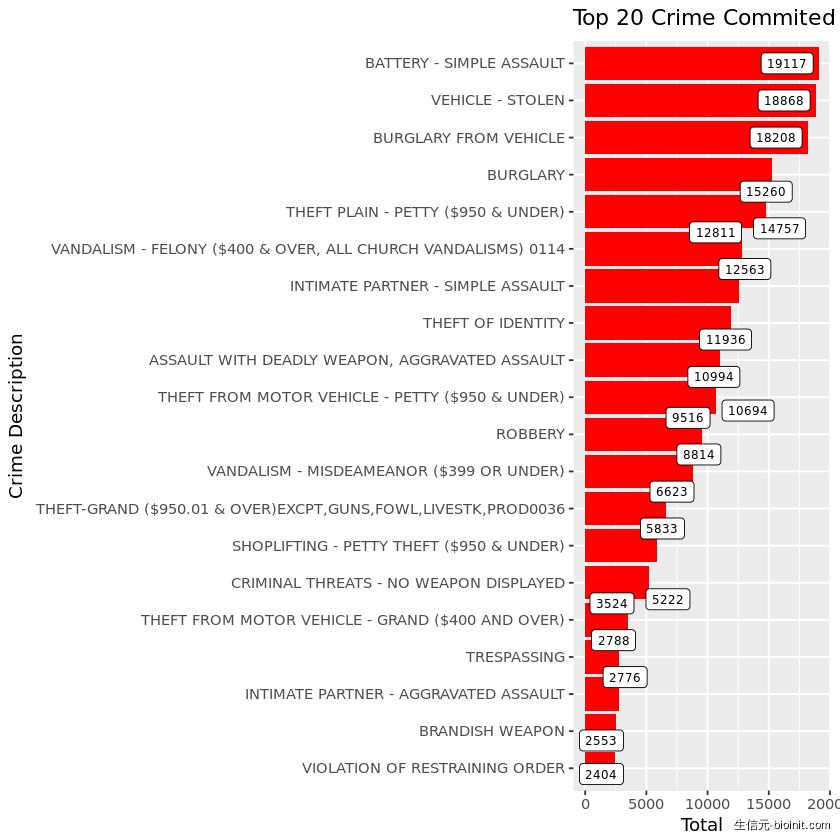

正如你所看到的，在 2017 犯下的大多数罪行是 battery-simple assault，车辆被盗（vehicle stolen）和车内盗窃（burglary from a vehicle）。

Age group

接下来，我将调查最有可能成为犯罪受害者的年龄组。

age <- year_2017 %>%
  group_by(`Victim Age`) %>%
  summarise(total = n()) %>%
  na.omit()

age %>%
  ggplot(aes(x = `Victim Age`, y = total)) +
  geom_line(group = 1) +
  geom_point(size = 0.5) +
  labs(title = "Age Most Likely To Become Crime Victim", 
       x = "Victim Age", 
       y = "Total")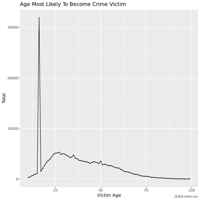

如上所述，年龄在 25 岁以下的人群最有可能成为 2017 的犯罪受害者。线条飙升最大的（huge spike）表示为 16 岁。

接下来，我将把年龄分为不同的组，并检查哪些犯罪是针对不同年龄组的。我将年龄组分为青少年（10-18岁）、青年（19—35岁）、中年（35-55岁）和老年人（56岁以上）。

year_2017$age_group <- cut(year_2017$`Victim Age`, breaks = c(-Inf, 19, 35, 55, Inf), labels = c("Teenager", "Young Adult", "Middle Age", "Elderly"))

age.group <- year_2017 %>%
  group_by(age_group, `Crime Code Description`) %>%
  summarise(total = n()) %>%
  top_n(20) %>%
  na.omit()

age.group %>%
  ggplot(aes(reorder(x = `Crime Code Description`, total), y = total)) +
  geom_col(fill = 'red') +
  geom_text(aes(label=total), color='black', hjust = -0.1, size = 3) +
  coord_flip() +
  facet_wrap(~ age_group) +
  labs(x = 'Total', 
       y = "Crime Description")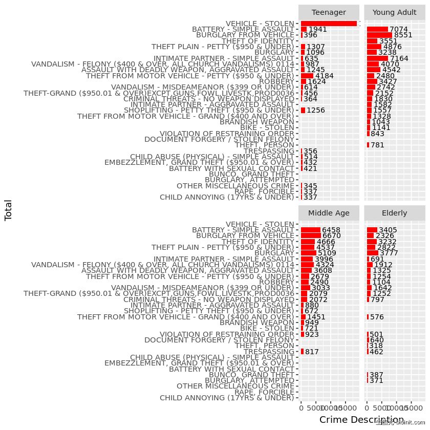

可以看出，不同年龄段的犯罪对象不同。

Gender

在这一节中，我将研究针对不同性别的犯罪类型。

gender <- year_2017 %>%
  group_by(`Victim Sex`, `Crime Code Description`) %>%
  summarise(total = n()) %>%
  filter(`Victim Sex` != "Unknown", `Victim Sex` != "H") %>%
  na.omit() %>%
  top_n(20) 

gender <- gender[-c(1:30),]

gender %>%
  ggplot(aes(reorder(x = `Crime Code Description`, total), y = total)) +
  geom_col(fill = 'green') +
  geom_text(aes(label=total), color='black', hjust = 0.8, size = 3) +
  coord_flip() +
  facet_wrap(~ `Victim Sex`) +
  labs(x = 'Total', 
       y = "Crime Description")

正如你所看到的，两性都可能是不同类型犯罪的受害者。

Map The Crime

接下来我们将对犯罪进行地图绘制。为了便于说明，我将只绘制 2017 年所犯的犯罪率最高的地图，这些犯罪行为是车辆被盗和车内盗窃。

#get the map of LA
LA_map <- qmap(location = "Los Angeles", zoom = 12)

#unfactor variable
year_2017$lat <- unfactor(year_2017$lat)
year_2017$long <- unfactor(year_2017$long)

#select relevant variables
mapping <- year_2017 %>%
  select(`Crime Code Description`, long, lat) %>%
  filter(`Crime Code Description` == 'BATTERY - SIMPLE ASSAULT') %>%
  na.omit()

#mapping
LA_map + geom_density_2d(aes(x = long, y = lat), data = mapping) +
  stat_density2d(data = mapping, 
    aes(x = long, y = lat, fill = ..level.., alpha = ..level..), size = 0.01, 
    bins = 16, geom = "polygon") + scale_fill_gradient(low = "green", high = "red", 
    guide = FALSE) + scale_alpha(range = c(0, 0.3), guide = FALSE)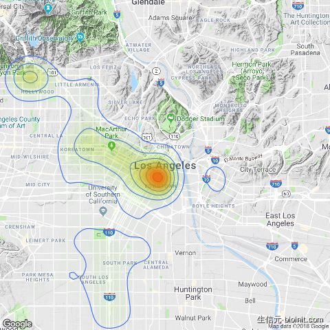

正如你所看到的，battery assault 更可能发生在洛杉矶市中心。

mapping <- year_2017 %>%
  select(`Crime Code Description`, long, lat) %>%
  filter(`Crime Code Description` == 'VEHICLE - STOLEN') %>%
  na.omit()

LA_map + geom_density_2d(aes(x = long, y = lat), data = mapping) +
  stat_density2d(data = mapping, 
    aes(x = long, y = lat, fill = ..level.., alpha = ..level..), size = 0.01, 
    bins = 16, geom = "polygon") + scale_fill_gradient(low = "green", high = "red", 
    guide = FALSE) + scale_alpha(range = c(0, 0.3), guide = FALSE)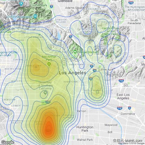

有趣的是，大多数车辆在洛杉矶南部更容易被盗。

mapping <- year_2017 %>%
  select(`Crime Code Description`, long, lat) %>%
  filter(`Crime Code Description` == 'BURGLARY FROM VEHICLE') %>%
  na.omit()

LA_map + geom_density_2d(aes(x = long, y = lat), data = mapping) +
  stat_density2d(data = mapping, 
    aes(x = long, y = lat, fill = ..level.., alpha = ..level..), size = 0.01, 
    bins = 16, geom = "polygon") + scale_fill_gradient(low = "green", high = "red", 
    guide = FALSE) + scale_alpha(range = c(0, 0.3), guide = FALSE)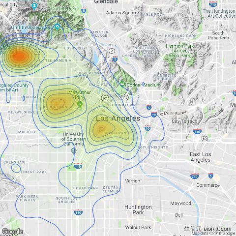

热图显示好莱坞，韩国城和洛杉矶市中心最有可能发生车内盗窃（burgalry from vehicle）。

结论

这只是一个简单的演示，说明如何深入了解数据并绘制位于洛杉矶的犯罪地图。

写在最后

这是一篇关于 R 深入了解数据、数据处理、数据（地图）可视化非常好的练习教程。整个操作脉络清晰、操作也不算难，推荐感兴趣的可以深入了解其中的一些操作原理，举一反三。

本文使用的数据：http://resource-1251708715.cosgz.myqcloud.com/r-example-data/Crime_Data_from_2010_to_Present.csv

原文：https://datascienceplus.com/analysis-of-los-angeles-crime-with-r/ 

作者：Chi Ting Low | 编译：Steven Shen

·end·

—如果喜欢，快分享给你的朋友们吧—

我们一起愉快的玩耍吧

本文分享自微信公众号 - 生信科技爱好者（bioitee）。
如有侵权，请联系 support@oschina.cn 删除。
本文参与“OSC源创计划”，欢迎正在阅读的你也加入，一起分享。