R 语言中的高级图像处理包
最新的 magick 包是为能够在 R 中更现代化、简单化高质量图像处理而进行的一次努力。该包封装了目前最强大的开源图片处理库 ImageMagick STL 。
ImageMagick 库具有大量功能。当前版本的 Magick 公开了很多内容,但是作为第一个发行版本,文档仍然很少。本文简单的介绍了其中一些最重要的概念来帮助了解 magick 。
安装 magick
在 Windows 或者 MacOS,可以通过 CRAN 安装该软件包。
install.packages("magick")
二进制 CRAN 软件包开箱即用,只需少量的工作,就可以使绝大多数的重要特性得以实现。使用 magick_config 可以查看您的 ImageMagick 版本支持哪些功能和格式。
> library(magick)
Linking to ImageMagick 6.9.9.14
Enabled features: cairo, freetype, fftw, ghostscript, lcms, pango, rsvg, webp
Disabled features: fontconfig, x11
> str(magick::magick_config())
List of 21
 $ version           :Class 'numeric_version'  hidden list of 1
  ..$ : int [1:4] 6 9 9 14
 $ modules           : logi FALSE
 $ cairo             : logi TRUE
 $ fontconfig        : logi FALSE
 $ freetype          : logi TRUE
 $ fftw              : logi TRUE
 $ ghostscript       : logi TRUE
 $ jpeg              : logi TRUE
 $ lcms              : logi TRUE
 $ libopenjp2        : logi FALSE
 $ lzma              : logi TRUE
 $ pangocairo        : logi TRUE
 $ pango             : logi TRUE
 $ png               : logi TRUE
 $ rsvg              : logi TRUE
 $ tiff              : logi TRUE
 $ webp              : logi TRUE
 $ wmf               : logi FALSE
 $ x11               : logi FALSE
 $ xml               : logi TRUE
 $ zero-configuration: logi TRUE
源码编译
Linux 下你需要安装 ImageMagick++ 库。在 Debian/Ubuntu,这个库叫 libmagick++-dev:
sudo apt-get install libmagick++-dev
在 Fedora 或者 CentOS/RHEL 我们需要安装 ImageMagick-c++-devel:
sudo yum install ImageMagick-c++-devel
要从 macOS 上的源代码安装,您需要来自 homebrew 的 imagemagick@6 。
brew install imagemagick@6
不幸的是,当前 homebrew 上的 imagemagick@6 配置禁用了许多功能,包括 librsvg 和 fontconfig。因此,字体和 svg 渲染的质量可能不是最佳的(建议安装时至少加上 --with-fontconfig 和 --with-librsvg 选项来支持高质量的字体和 svg 渲染。CRAN 上的 OS-Xe 二进制包已经默认配置好了)。
图像输入输出
magick 之所以如此神奇,是因为它会自动转换并呈现所有常见的图像格式。ImageMagick 支持数十种格式并自动检测类型。使用 magick::magick_config() 可以列出您的 ImageMagick 版本支持的格式。
读和写
可以使用 image_read 从图像数据的文件路径,URL 或原始矢量直接读取图像。image_info 函数显示有关图像的一些元数据,类似 于 imagemagick 标识命令行实用程序。
library(magick)
tiger <- image_read_svg('http://jeroen.github.io/images/tiger.svg', width = 350)
print(tiger)
##   format width height colorspace matte filesize density
## 1    PNG   350    350       sRGB  TRUE        0   72x72

我们使用 image_write 将任何格式的图像导出为磁盘上的文件,或者如果 path = NULL 则导出到内存中的文件。
# Render svg to png bitmap
image_write(tiger, path = "tiger.png", format = "png")
如果 path 是文件名,则 image_write 成功返回 path,以便可以将结果通过文件路径传递给函数。
转换格式
Magick 以原始格式将图像保留在内存中。你可以在 image_write 中通过指定格式参数以转换为另一种格式。或者还可以在应用转换之前,先在内部将图像转换为其他格式。如果你的原始格式是有损的,这将很有用。
tiger_png <- image_convert(tiger, "png")
image_info(tiger_png)
##   format width height colorspace matte filesize density
## 1    PNG   350    350       sRGB  TRUE        0   72x72
预览
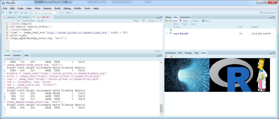
具有内置网络浏览器(例如 RStudio)的 IDE 会在查看器中自动显示魔术图像。这就形成了一个整洁的交互式图像编辑环境。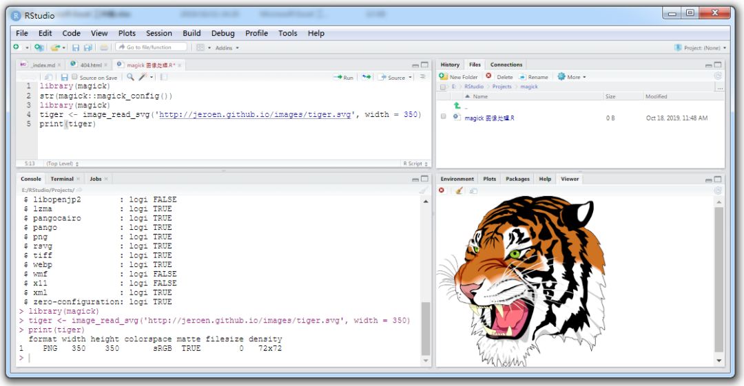
另外,在 Linux 上,您可以使用 image_display 在 X11 窗口中预览图像。最后,image_browse 会在你系统默认的应用程序中为给定类型打开图像。
# X11 only
image_display(tiger)

# System dependent
image_browse(tiger)
另一种方法是将图像转换为栅格对象,然后将其绘制在 R 的图形显示上。但是,这非常慢,并且仅在与其他绘图功能结合使用时才有用。
转变
了解可用转换的最佳方法是遍历 RStudio中 ?transformations 页面中的示例。下面是一些示例。
剪切与编辑
一些转换函数采用了 geometry 参数,该参数需要 AxB + C + D 形式的特殊语法,其中每个元素都是可选的。一些例子:
image_crop(image, "100x150+50"): crop outwidth:100pxandheight:150pxstarting+50pxfrom the leftimage_scale(image, "200"): resize proportionally to width:200pximage_scale(image, "x200"): resize proportionally to height:200pximage_fill(image, "blue", "+100+200"): flood fill with blue starting at the point atx:100, y:200image_border(frink, "red", "20x10"): adds a border of 20px left+right and 10px top+bottom
完整的语法,可以参考 Magick::Geometry 文档。
# Example image
frink <- image_read("https://jeroen.github.io/images/frink.png")
print(frink)
##   format width height colorspace matte filesize density
## 1    PNG   220    445       sRGB  TRUE    73494   72x72

# Add 20px left/right and 10px top/bottom
image_border(image_background(frink, "hotpink"), "#000080", "20x10")

# Trim margins
image_trim(frink)

# Passport pica
image_crop(frink, "100x150+50")

# Resize
image_scale(frink, "300") # width: 300px

image_scale(frink, "x300") # height: 300px

# Rotate or mirror
image_rotate(frink, 45)

image_flip(frink)

image_flop(frink)

# Brightness, Saturation, Hue
image_modulate(frink, brightness = 80, saturation = 120, hue = 90)

# Paint the shirt orange
image_fill(frink, "orange", point = "+100+200", fuzz = 20)

使用 image_fill,我们可以从像素点开始填充。模糊参数允许填充物穿过具有相似颜色的相邻像素。值必须在 0 到 256^2 之间,指定要视为相等的颜色之间的最大几何距离。在这里,我们给教授 Frink 一件橙色的世界杯衬衫。
滤镜和效果
ImageMagick 还具有许多值得去检查尝试的标准效果。
# Add randomness
image_blur(frink, 10, 5)

image_noise(frink)

# Silly filters
image_charcoal(frink)

image_oilpaint(frink)

image_negate(frink)

核卷积
image_convolve() 函数在图像上实行 kernel 变换。核卷积是指在核矩阵中,图片每个像素的值根据相邻像素的加权和重新计算。例如,让我们看一下这个简单的核变换:
kern <- matrix(0, ncol = 3, nrow = 3)
kern[1, 2] <- 0.25
kern[2, c(1, 3)] <- 0.25
kern[3, 2] <- 0.25
kern
##      [,1] [,2] [,3]
## [1,] 0.00 0.25 0.00
## [2,] 0.25 0.00 0.25
## [3,] 0.00 0.25 0.00
该核变换将每个像素更改为其水平和垂直相邻像素的平均值,从而在下面的右侧图像中产生轻微的模糊效果:
img <- image_resize(logo, "300x300")
img_blurred <- image_convolve(img, kern)
image_append(c(img, img_blurred))

或使用任何的 standard kernels:
img %>% image_convolve('Sobel') %>% image_negate()

img %>% image_convolve('DoG:0,0,2') %>% image_negate()

文本注释
最后,在图像的最上层打印输出一些文本往往是十分有用的:
# Add some text
image_annotate(frink, "bioinit", size = 70, gravity = "southwest", color = "green")

# Customize text
image_annotate(frink, "Welcome to bioinit", size = 30, color = "red", boxcolor = "pink",
  degrees = 60, location = "+50+100")

# Fonts may require ImageMagick has fontconfig
image_annotate(frink, "Hello world, bioinit!", font = 'Times', size = 30)

大多数平台上支持的字体,包括 "sans", "mono", "serif", "Times", "Helvetica", "Trebuchet", "Georgia", "Palatino" ,以及 "Comic Sans" 。
与管道结合
每个图像转换功能都会返回一个原始图像的修改后的副本。它不会影响原始图像。
frink <- image_read("https://jeroen.github.io/images/frink.png")
frink2 <- image_scale(frink, "100")
image_info(frink)
##   format width height colorspace matte filesize density
## 1    PNG   220    445       sRGB  TRUE    73494   72x72
image_info(frink2)
##   format width height colorspace matte filesize density
## 1    PNG   100    202       sRGB  TRUE        0   72x72
因此,要组合转换,你需要将它们链接起来:
test <- image_rotate(frink, 90)
test <- image_background(test, "blue", flatten = TRUE)
test <- image_border(test, "red", "10x10")
test <- image_annotate(test, "This is how we combine transformations", color = "white", size = 30)
print(test)
##   format width height colorspace matte filesize density
## 1    PNG   465    240       sRGB  TRUE        0   72x72

使用 magrittr 管道语法,可以使这一过程更具可读性。
image_read("https://jeroen.github.io/images/frink.png") %>%
  image_rotate(270) %>%
  image_background("blue", flatten = TRUE) %>%
  image_border("red", "10x10") %>%
  image_annotate("The same thing with pipes", color = "white", size = 30)

图像向量
上面的示例涉及的是单个图像。但是,Magick 中的所有函数都已经过向量化,以支持图层、合成或动画的处理。
标准的基本方法 [ ,[[,c() 和 length() 可用于处理图像向量,然后可以将其视为图层或帧。
# Download earth gif and make it a bit smaller for vignette
earth <- image_read("https://jeroen.github.io/images/earth.gif") %>%
  image_scale("200x") %>%
  image_quantize(128)

length(earth)
## [1] 44
earth

head(image_info(earth))
##   format width height colorspace matte filesize density
## 1    GIF   200    200        RGB FALSE        0   72x72
## 2    GIF   200    200        RGB FALSE        0   72x72
## 3    GIF   200    200        RGB FALSE        0   72x72
## 4    GIF   200    200        RGB FALSE        0   72x72
## 5    GIF   200    200        RGB FALSE        0   72x72
## 6    GIF   200    200        RGB FALSE        0   72x72
rev(earth) %>%
  image_flip() %>%
  image_annotate("meanwhile in Australia", size = 20, color = "white")

图层
我们可以像在 Photoshop 中那样,将图层堆叠在一起:
bigdata <- image_read('https://jeroen.github.io/images/bigdata.jpg')
frink <- image_read("https://jeroen.github.io/images/frink.png")
logo <- image_read("https://jeroen.github.io/images/Rlogo.png")
img <- c(bigdata, logo, frink)
img <- image_scale(img, "300x300")
image_info(img)
##   format width height colorspace matte filesize density
## 1   JPEG   300    225       sRGB FALSE        0   72x72
## 2    PNG   300    232       sRGB  TRUE        0   72x72
## 3    PNG   148    300       sRGB  TRUE        0   72x72
打印的图案相互镶嵌叠加在一起,从而扩展输出画布,使所有内容都适合:
image_mosaic(img)

Flattening 扁平化处理将各个图层合并成一张与第一张图片大小相同的图片:
image_flatten(img)

Flattening 和 mosaic 处理允许指定其他的复合运算符操作(composite operators):
image_flatten(img, 'Add')

image_flatten(img, 'Modulate')

image_flatten(img, 'Minus')

合并
Appending 追加意味着将框架彼此相邻放置:
image_append(image_scale(img, "x200"))

使用 stack = TRUE 可以将它们放置在彼此的顶部:
image_append(image_scale(img, "100"), stack = TRUE)

合成允许在特定位置上组合两个图像:
bigdatafrink <- image_scale(image_rotate(image_background(frink, "none"), 300), "x200")
image_composite(image_scale(bigdata, "x400"), bigdatafrink, offset = "+180+100")

页面
当读取 PDF 文档时,每个页面都成为向量的一个元素。注意,PDF 是在读取时呈现的,因此需要立即指定密度。
manual <- image_read_pdf('https://cloud.r-project.org/web/packages/magick/magick.pdf', density = 72)
image_info(manual)
##    format width height colorspace matte filesize density
## 1     PNG   612    792       sRGB  TRUE        0   72x72
## 2     PNG   612    792       sRGB  TRUE        0   72x72
## 3     PNG   612    792       sRGB  TRUE        0   72x72
## 4     PNG   612    792       sRGB  TRUE        0   72x72
## 5     PNG   612    792       sRGB  TRUE        0   72x72
## 6     PNG   612    792       sRGB  TRUE        0   72x72
## 7     PNG   612    792       sRGB  TRUE        0   72x72
## 8     PNG   612    792       sRGB  TRUE        0   72x72
## 9     PNG   612    792       sRGB  TRUE        0   72x72
## 10    PNG   612    792       sRGB  TRUE        0   72x72
## 11    PNG   612    792       sRGB  TRUE        0   72x72
## 12    PNG   612    792       sRGB  TRUE        0   72x72
## 13    PNG   612    792       sRGB  TRUE        0   72x72
## 14    PNG   612    792       sRGB  TRUE        0   72x72
## 15    PNG   612    792       sRGB  TRUE        0   72x72
## 16    PNG   612    792       sRGB  TRUE        0   72x72
## 17    PNG   612    792       sRGB  TRUE        0   72x72
## 18    PNG   612    792       sRGB  TRUE        0   72x72
## 19    PNG   612    792       sRGB  TRUE        0   72x72
## 20    PNG   612    792       sRGB  TRUE        0   72x72
## 21    PNG   612    792       sRGB  TRUE        0   72x72
## 22    PNG   612    792       sRGB  TRUE        0   72x72
## 23    PNG   612    792       sRGB  TRUE        0   72x72
## 24    PNG   612    792       sRGB  TRUE        0   72x72
## 25    PNG   612    792       sRGB  TRUE        0   72x72
## 26    PNG   612    792       sRGB  TRUE        0   72x72
## 27    PNG   612    792       sRGB  TRUE        0   72x72
## 28    PNG   612    792       sRGB  TRUE        0   72x72
## 29    PNG   612    792       sRGB  TRUE        0   72x72
## 30    PNG   612    792       sRGB  TRUE        0   72x72
## 31    PNG   612    792       sRGB  TRUE        0   72x72
## 32    PNG   612    792       sRGB  TRUE        0   72x72
## 33    PNG   612    792       sRGB  TRUE        0   72x72
## 34    PNG   612    792       sRGB  TRUE        0   72x72
## 35    PNG   612    792       sRGB  TRUE        0   72x72
manual[1]

动画
除了将矢量元素视为图层之外,我们还可以将它们制作成动画帧!
image_animate(image_scale(img, "200x200"), fps = 1, dispose = "previous")

变形创建了 n 个图像序列,这些序列逐渐地将一个图像变形为另一个图像。这样,它就变成了动画。
newlogo <- image_scale(image_read("https://jeroen.github.io/images/Rlogo.png"), "x150")
oldlogo <- image_scale(image_read("https://developer.r-project.org/Logo/Rlogo-3.png"), "x150")
frames <- image_morph(c(oldlogo, newlogo), frames = 10)
image_animate(frames)

如果您读入现有的 GIF 或视频文件,则每一帧都会变成一个图层:
# Foreground image
banana <- image_read("https://jeroen.github.io/images/banana.gif")
banana <- image_scale(banana, "150")
image_info(banana)
##   format width height colorspace matte filesize density
## 1    GIF   150    148       sRGB  TRUE        0   72x72
## 2    GIF   150    148       sRGB  TRUE        0   72x72
## 3    GIF   150    148       sRGB  TRUE        0   72x72
## 4    GIF   150    148       sRGB  TRUE        0   72x72
## 5    GIF   150    148       sRGB  TRUE        0   72x72
## 6    GIF   150    148       sRGB  TRUE        0   72x72
## 7    GIF   150    148       sRGB  TRUE        0   72x72
## 8    GIF   150    148       sRGB  TRUE        0   72x72
处理各个帧并将其放回动画中:
# Background image
background <- image_background(image_scale(logo, "200"), "white", flatten = TRUE)

# Combine and flatten frames
frames <- image_composite(background, banana, offset = "+70+30")

# Turn frames into animation
animation <- image_animate(frames, fps = 10)
print(animation)
##   format width height colorspace matte filesize density
## 1    gif   200    155       sRGB  TRUE        0   72x72
## 2    gif   200    155       sRGB  TRUE        0   72x72
## 3    gif   200    155       sRGB  TRUE        0   72x72
## 4    gif   200    155       sRGB  TRUE        0   72x72
## 5    gif   200    155       sRGB  TRUE        0   72x72
## 6    gif   200    155       sRGB  TRUE        0   72x72
## 7    gif   200    155       sRGB  TRUE        0   72x72
## 8    gif   200    155       sRGB  TRUE        0   72x72

动画可以另存为 GIF 格式的 MPEG 文件:
image_write(animation, "Rlogo-banana.gif")
绘图与图形
该软件包的一个相对较新的组件是一个本地的 R 图形设备,它生成 magick 图像对象。它可以像用于绘制绘图的常规设备一样使用它,也可以打开一个使用像素坐标绘制到现有图像的设备。
图形设备
image_graph() 函数可打开一个新的图形设备,类似于 png() 或 x11() 。它返回要写入绘图的图像对象。绘图设备中的每个“page”都将成为图像对象中的一帧。
# Produce image using graphics device
fig <- image_graph(width = 400, height = 400, res = 96)
ggplot2::qplot(mpg, wt, data = mtcars, colour = cyl)
dev.off()
我们可以使用常规图像操作轻松地对图形进行后处理。
# Combine
out <- image_composite(fig, frink, offset = "+70+30")
print(out)
## # A tibble: 1 x 7
##   format width height colorspace matte filesize density
##   <chr>  <int>  <int> <chr>      <lgl>    <int> <chr>
## 1 PNG      400    400 sRGB       TRUE         0 72x72

绘图设备
使用图形设备的另一种方法是使用像素坐标在现有图像的上面绘制。
# Or paint over an existing image
img <- image_draw(frink)
rect(20, 20, 200, 100, border = "red", lty = "dashed", lwd = 5)
abline(h = 300, col = 'blue', lwd = '10', lty = "dotted")
text(30, 250, "Hoiven-Glaven", family = "monospace", cex = 4, srt = 90)
palette(rainbow(11, end = 0.9))
symbols(rep(200, 11), seq(0, 400, 40), circles = runif(11, 5, 35),
  bg = 1:11, inches = FALSE, add = TRUE)
dev.off()
print(img)
## # A tibble: 1 x 7
##   format width height colorspace matte filesize density
##   <chr>  <int>  <int> <chr>      <lgl>    <int> <chr>
## 1 PNG      220    445 sRGB       TRUE         0 72x72

默认情况下,image_draw() 将所有空白设置为 0,并使用图形坐标来匹配图像大小,像素(宽度x高度)为左上角 (0,0)。注意,这意味着 y 轴从上到下递增,这与典型的图形坐标相反。您可以通过向 image_draw 传递定制的 xlim、ylim 或 mar 值来覆盖所有这些。
动画图形
图形设备支持多帧,这使它很容易创建动画图形。下面的代码展示了如何使用 magick 图形设备实现来自非常酷的 gganimate 包的示例。
library(gapminder)
library(ggplot2)
img <- image_graph(600, 340, res = 96)
datalist <- split(gapminder, gapminder$year)
out <- lapply(datalist, function(data){
  p <- ggplot(data, aes(gdpPercap, lifeExp, size = pop, color = continent)) +
    scale_size("population", limits = range(gapminder$pop)) + geom_point() + ylim(20, 90) +
    scale_x_log10(limits = range(gapminder$gdpPercap)) + ggtitle(data$year) + theme_classic()
  print(p)
})
dev.off()
animation <- image_animate(img, fps = 2)
print(animation)
## # A tibble: 12 x 7
##    format width height colorspace matte filesize density
##    <chr>  <int>  <int> <chr>      <lgl>    <int> <chr>
##  1 gif      600    340 sRGB       TRUE         0 72x72
##  2 gif      600    340 sRGB       TRUE         0 72x72
##  3 gif      600    340 sRGB       TRUE         0 72x72
##  4 gif      600    340 sRGB       TRUE         0 72x72
##  5 gif      600    340 sRGB       TRUE         0 72x72
##  6 gif      600    340 sRGB       TRUE         0 72x72
##  7 gif      600    340 sRGB       TRUE         0 72x72
##  8 gif      600    340 sRGB       TRUE         0 72x72
##  9 gif      600    340 sRGB       TRUE         0 72x72
## 10 gif      600    340 sRGB       TRUE         0 72x72
## 11 gif      600    340 sRGB       TRUE         0 72x72
## 12 gif      600    340 sRGB       TRUE         0 72x72

要将其写入文件,您只需执行以下操作:
image_write(animation, "gapminder.gif")
光栅图像
Magick 图像也可以转换为光栅对象,来用于 R 的图形设备。因此,我们可以将它与其他图形工具相结合。然而,请注意,R 的图形设备非常慢,且它有一个非常不同的坐标系,它会降低图像的质量。
基础格栅
Base R 有一个 as.raster 格式,它可将图像转换为字符串向量。Paul Murrell 在 Raster Images in R Graphics 一文中给出了一个很好的概述。
plot(as.raster(frink))

# Print over another graphic
plot(cars)
rasterImage(frink, 21, 0, 25, 80)

grid 包
grid 包使您更容易在图形设备上叠加栅格,而不必调整绘图的 x/y 坐标。
library(ggplot2)
library(grid)
qplot(speed, dist, data = cars, geom = c("point", "smooth"))
## `geom_smooth()` using method = 'loess' and formula 'y ~ x'
grid.raster(frink)

raster 包
raster 包具有自己的 bitmaps 类,这些类对于空间应用程序很有用。将图像转换为栅格的最简单方法是将其导出为 tiff 文件:
tiff_file <- tempfile()
image_write(frink, path = tiff_file, format = 'tiff')
r <- raster::brick(tiff_file)
raster::plotRGB(r)

你还可以手动将位图数组(bitmap array )转换为栅格对象,但这似乎会删除一些元数据:
buf <- as.integer(frink[[1]])
rr <- raster::brick(buf)
raster::plotRGB(rr, asp = 1)
OCR 文本提取
magick 最新的功能是利用 OCR 技术从图片中提取文本。这需要 tesseract 包。
install.packages("tesseract")
img <- image_read("http://jeroen.github.io/images/testocr.png")
print(img)
## # A tibble: 1 x 7
##   format width height colorspace matte filesize density
##   <chr>  <int>  <int> <chr>      <lgl>    <int> <chr>
## 1 PNG      640    480 sRGB       TRUE     23359 72x72

# Extract text
cat(image_ocr(img))
## This is a lot of 12 point text to test the
## ocr code and see if it works on all types
## of file format.
##
## The quick brown dog jumped over the
## lazy fox. The quick brown dog jumped
## over the lazy fox. The quick brown dog
## jumped over the lazy fox. The quick
## brown dog jumped over the lazy fox.
总结
本文章篇幅很长,对 magick 包的各种使用非常直观详细。作为与 ImageMagick 绑定,可用的最全面的开源图像处理库,magick 包支持许多常见格式(png,jpeg,tiff,pdf 等)和操作(旋转,缩放,修剪,修剪,翻转,模糊等)。这些所有操作都是通过 Magick ++ STL 矢量化的,这意味着它们可以在单个帧或一系列帧上进行操作,以处理图层,拼贴或动画。
在 RStudio 中,可以将图像打印到控制台后会自动预览,从而形成一个交互式编辑环境。因此,强烈推荐大家在 RStudio 中进行使用和测试。
更多 magick、ImageMagick 相关的 R 语言高级图像处理操作,有兴趣的童鞋可以自行去研究学习,也欢迎大家留言交流。
参考资料:
https://cran.r-project.org/web/packages/magick/vignettes/intro.html
——The End——

本文分享自微信公众号 - 生信科技爱好者(bioitee)。
如有侵权,请联系 support@oschina.cn 删除。
本文参与“OSC源创计划”,欢迎正在阅读的你也加入,一起分享。
