【深度学习 01】线性回归+PyTorch实现

1. 线性回归
2. 从零实现线性回归
3. 使用深度学习框架（PyTorch）实现线性回归
4. 报错总结
参考资料

回到顶部

1. 线性回归

1.1 线性模型

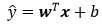
当输入包含d个特征，预测结果表示为：

记x为样本的特征向量，w为权重向量，上式可表示为：

对于含有n个样本的数据集，可用X来表示n个样本的特征集合，其中行代表样本，列代表特征，那么预测值可用矩阵乘法表示为：

给定训练数据特征X和对应的已知标签y，线性回归的⽬标是找到⼀组权重向量w和偏置b：当给定从X的同分布中取样的新样本特征时，这组权重向量和偏置能够使得新样本预测标签的误差尽可能小。

1.2 损失函数（loss function）

损失函数又称代价函数（cost function），通常用其来度量目标的实际值和预测值之间的误差。在回归问题中，常用的损失函数为平方误差函数：

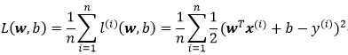
我们的目标便是求得最小化损失函数下参数w和b的值：

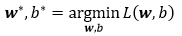
求解上式，一般有以下两种方式：

1> 正规方程（解析解）

2> 梯度下降（gradient descent）

（1）初始化模型参数的值，如随机初始化；

（2）从数据集中随机抽取小批量样本且在负梯度的方向上更新参数，并不断迭代这一步骤。

上式中：n表示每个小批量中的样本数，也称批量大小（batch size）、α表示学习率（learning rate），n和α的值需要手动预先指定，而不是模型训练得到的，这类参数称为超参数（hyperparameter），选择超参数的过程称为调参（hyperparameter tuning)。

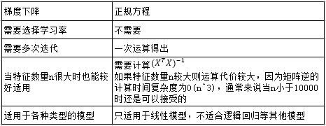
梯度下降和正规方程比较：

1.3 矢量化加速

为了加快模型训练速度，可以采用矢量化计算的方式，这通常会带来数量级的加速。下边用代码简单对比测试下矢量化计算的加速效果。

import math
import time
import numpy as np
import torch
from d2l import torch as d2l
 
# a、b是全为1的10000维向量
n = 10000
a = torch.ones(n)
b = torch.ones(n)
 
 
class Timer:
    def __init__(self):
        """记录多次运行时间"""
        self.tik = None
        self.times = []
        self.start()
 
    def start(self):
        """启动计时器"""
        self.tik = time.time()
 
    def stop(self):
        """停止计时器并将时间记录在列表中"""
        self.times.append(time.time() - self.tik)
        return self.times[-1]
 
    def avg(self):
        """返回平均时间"""
        return sum(self.times) / len(self.times)
 
    def sum(self):
        """返回总时间"""
        return sum(self.times)
 
    def cumsum(self):
        """返回总时间"""
        return np.array(self.times).cumsum().tolist()
 
 
c = torch.zeros(n)
timer = Timer()
for i in range(n):
    c[i] = a[i] + b[i]
print(f'{timer.stop():.5f} sec')
 
timer.start()
d = a + b
print(f'{timer.stop():.5f} sec')　　

代码运行结果如下，可见矢量化代码确实极大的提高了计算速度。

注：这里矢量化计算d=a+b的时间不知道为什么统计出来是0，可能是跟电脑的计时器精度有关。

回到顶部

2. 从零实现线性回归

线性回归的实现过程可以简单总结为以下几个步骤：

（1）读取数据（或构造数据），转换成需要的格式和类型，并生成标签；

（2）定义初始化模型参数、定义模型、定义损失函数、定义优化算法；

（3）使用优化算法训练模型。

import random
import torch
import numpy as np
from matplotlib import pyplot as plt
from d2l import torch as d2l
 
 
# 构造数据集
def synthetic_data(w, b, num_examples):
    """生成 y = Xw + b + 噪声。"""
    # 均值为0，方差为1的随机数，行数为样本数，列数是w的长度(行代表样本，列代表特征）
    X = torch.normal(0, 1, (num_examples, len(w)))  # pytorch较新版本
    # X = torch.tensor(np.random.normal(0, 1, (num_examples, len(w))), dtype=torch.float32)  # pytorch1.1.0版本
    y = torch.matmul(X, w) + b
    # 均值为0，方差为1的随机数，噪声项。
    y += torch.normal(0, 0.01, y.shape)  # pytorch较新版本
    # y += torch.tensor(np.random.normal(0, 0.01, y.shape), dtype=torch.float32)  # pytorch1.1.0版本
    return X, y.reshape((-1, 1))
 
 
true_w = torch.tensor([2, -3.4])
true_b = 4.2
features, labels = synthetic_data(true_w, true_b, 1000)
print('features:', features[0], '\nlabel:', labels[0])
 
d2l.set_figsize()
d2l.plt.scatter(features[:, 1].detach().numpy(), labels.detach().numpy(), 1)
 
 
# 生成一个data_iter函数，该函数接收批量大小、特征矩阵和标签向量作为输入，生成大小为batch_size的小批量
def data_iter(batch_size, features, labels):
    num_examples = len(features)
    indices = list(range(num_examples))
    # 这些样本是随机读取的，没有特定的顺序
    random.shuffle(indices)
    for i in range(0, num_examples, batch_size):
        batch_indices = torch.tensor(indices[i:min(i+batch_size, num_examples)])
        yield features[batch_indices], labels[batch_indices]
 
 
batch_size = 10
for X, y in data_iter(batch_size, features, labels):
    print(X, '\n', y)
    break
 
# 定义初始化模型参数
w = torch.normal(0, 0.01, size=(2, 1), requires_grad=True)  # pytorch较新版本
# w = torch.autograd.Variable(torch.tensor(np.random.normal(0, 0.01, size=(2, 1)),
#                                          dtype=torch.float32), requires_grad=True)  # pytorch1.1.0版本
b = torch.zeros(1, requires_grad=True)
 
 
# 定义模型
def linreg(X, w, b):
    """线性回归模型。"""
    return torch.matmul(X, w) + b
 
 
# 定义损失函数
def squared_loss(y_hat, y):
    """均方损失。"""
    return (y_hat - y.reshape(y_hat.shape))**2 / 2
 
 
# 定义优化算法
def sgd(params, lr, batch_size):
    """小批量随机梯度下降"""
    with torch.no_grad():
        for param in params:
            param -= lr * param.grad / batch_size
            param.grad.zero_()
 
 
# 训练过程
lr = 0.03
num_epochs = 3
net = linreg
loss = squared_loss
 
for epoch in range(num_epochs):
    for X, y in data_iter(batch_size, features, labels):
        l = loss(net(X, w, b), y)  # X和y的小批量损失
        # 因为l形状是（batch_size, 1），而不是一个标量。l中的所有元素被加到一起并以此来计算关于[w, b]的梯度
        l.sum().backward()
        sgd([w, b], lr, batch_size)  # 使用参数的梯度更新参数
    with torch.no_grad():
        train_l = loss(net(features, w, b), labels)
        print(f'epoch {epoch + 1}, loss {float(train_l.mean()):f}')
 
print(f'w的估计误差：{true_w - w.reshape(true_w.shape)}')
print(f'b的估计误差：{true_b - b}')　

回到顶部

3. 使用深度学习框架（PyTorch）实现线性回归

使用PyTorch封装的高级API可以快速高效的实现线性回归

import numpy as np
import torch
from torch import nn  # 'nn'是神经网路的缩写
from torch.utils import data
from d2l import torch as d2l
 
 
# 构造数据集
def synthetic_data(w, b, num_examples):
    """生成 y = Xw + b + 噪声。"""
    # 均值为0，方差为1的随机数，行数为样本数，列数是w的长度(行代表样本，列代表特征）
    X = torch.normal(0, 1, (num_examples, len(w)))  # pytorch较新版本
    # X = torch.tensor(np.random.normal(0, 1, (num_examples, len(w))), dtype=torch.float32)  # pytorch1.1.0版本
    y = torch.matmul(X, w) + b
    # 均值为0，方差为1的随机数，噪声项。
    y += torch.normal(0, 0.01, y.shape)  # pytorch较新版本
    # y += torch.tensor(np.random.normal(0, 0.01, y.shape), dtype=torch.float32)  # pytorch1.1.0版本
    return X, y.reshape((-1, 1))
 
 
true_w = torch.tensor([2, -3.4])
true_b = 4.2
features, labels = synthetic_data(true_w, true_b, 1000)
 
d2l.set_figsize()
d2l.plt.scatter(features[:, 1].detach().numpy(), labels.detach().numpy(), 1)
 
 
# 调用框架中现有的API来读取数据
def load_array(data_arrays, batch_size, is_train=True):
    """构造一个PyTorch数据迭代器"""
    dataset = data.TensorDataset(*data_arrays)
    return data.DataLoader(dataset, batch_size, shuffle=is_train)
 
 
batch_size = 10
data_iter = load_array((features, labels), batch_size)
 
print(next(iter(data_iter)))
 
# 使用框架预定义好的层
net = nn.Sequential(nn.Linear(2, 1))
 
# 初始化模型参数（等价于前边手动实现w、b以及network的方式）
net[0].weight.data.normal_(0, 0.01)  # 使用正态分布替换掉w的值
net[0].bias.data.fill_(0)
 
# 计算均方误差使用MSELoss类，也称为平方L2范数
loss = nn.MSELoss()
 
# 实例化SGD实例
trainer = torch.optim.SGD(net.parameters(), lr=0.03)
 
# 训练
num_epochs = 3  # 迭代三个周期
for epoch in range(num_epochs):
    for X, y in data_iter:
        l = loss(net(X), y)
        trainer.zero_grad()  # 优化器，先将梯度清零
        l.backward()
        trainer.step()  # 模型更新
    l = loss(net(features), labels)
    print(f'epoch {epoch + 1}, loss {l:f}')
 
w = net[0].weight.data
print('w的估计误差：', true_w - w.reshape(true_w.shape))
b = net[0].bias.data
print('b的估计误差：', true_b - b)

回到顶部

4. 报错总结

1. torch.normal()报错，这个是由于PyTorch版本问题，torch.normal()函数的参数形式和用法有所变化。

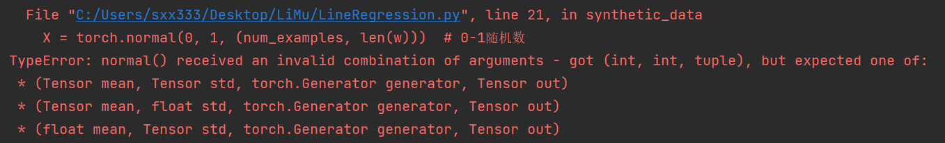
要生成均值为0且方差为1的随机数，pytorch1.1.0和pytorch1.9.0可以分别采用以下形式：

# pytorch1.9.0 
X = torch.normal(0, 1, (num_examples, len(w)))    
# pytorch1.1.0（也适用于高版本） 
X = torch.tensor(np.random.normal(0, 1, (num_examples, len(w))), dtype=torch.float32)

2. d2l库安装报错。这个我在公司电脑上直接一行pip install d2l成功安装，回家换自己电脑，各种报错。解决之后发现大多都是找不到安装源、缺少相关库或者库版本不兼容的问题。

安装方式：conda install d2l 或 pip install d2l。网速太慢下不下来可以选择国内源镜像：

1	`pip install d2l` `-i http://pypi.douban.com/simple/` `--trusted-host pypi.douban.com`

国内常用源镜像：

# 清华：https://pypi.tuna.tsinghua.edu.cn/simple
# 阿里云：http://mirrors.aliyun.com/pypi/simple/
# 中国科技大学 https://pypi.mirrors.ustc.edu.cn/simple/
# 华中理工大学：http://pypi.hustunique.com/
# 山东理工大学：http://pypi.sdutlinux.org/
# 豆瓣：http://pypi.douban.com/simple/ 

需要注意的是：有时候使用conda install d2l命令无法下载，改为pip 命令后即可下载成功。这是因为有些包只能通过pip安装。Anaconda提供超过1,500个软件包，包括最流行的数据科学、机器学习和AI框架，这与PyPI上提供的150,000多个软件包相比，只是一小部分。

Python官方安装whl包和tar.gz包安装方法：

安装whl包：pip install wheel，pip install xxx.whl

安装tar.gz包：cd到解压后路径，python setup.py install

回到顶部