GNN Visualization

Introduction

There are some traditional method for visualizing GNN and explanation system for it. But there is no specific visualization method for GNN. Based on the difference between GNN and other neural networks, there should be a specific method for GNN visualization.

Background

Machine learning task for graphs:

　　node classification

　　link prediction

　　graph classification

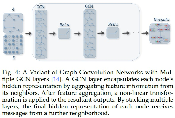
Here is a classical GNN model for node classification.

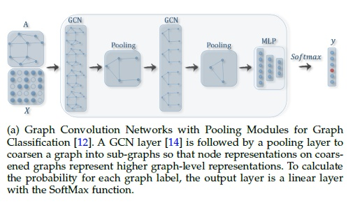
Here is a classical GNN model for graph classification.

Aims of visualization is to better understand how GNN helps to solve the tasks. So when doing visualization, they need to be dealed with separately. 

Graph Neural Network

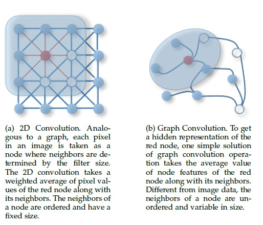
Similar to Convolutional Neural Network, GNN also learns the weights for every features and sum them. The difference is that GNN aggregate from local neighbor rather than two-dimensional matrix. For multi-layer GNN, it can gradually learn more abstract features with the increasement of layers. It can be represented as:

 

where W is the learning weight, A is adjacency matrix, H is hidden layer embeddings and σ is the activation function.  

We can also transform the learning processes into three parts: Transform, Aggregate and Update. All the variants of GNN consist of these three parts.

Transform:

　　Transform the current node features to new features, usually using weights (HW)

Aggregate:

　　Aggregate information from neighborhood and calculates an aggregated message via an aggregation method

Update:

　　Update the representation of l layer from l-1 layer non-linearly.

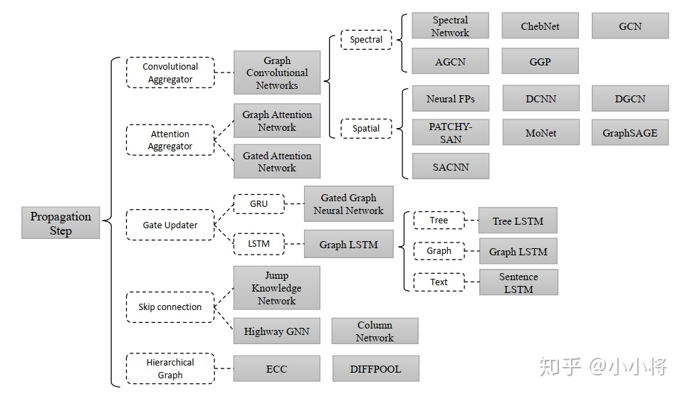
Here is a figure for GNN family.

Classical Neural Network Visualization Method

From the perspective of interpretability:

　　simple proxy models of full neural networks

　　　　linear models or sets of rules

　　　　model-agnostic way

　　identify important aspects of the computation

　　　　feature gradients

　　　　backpropagation of neurons’ contributions

　　　　counterfactual reasoning

　　attention mechanisms like GAT learned

　　　　edge attention values can indicate important graph structure, the values are the same for predictions across all nodes.

From the perspective of concrete technique:

　　Representation plotting (direct plotting, t-SNE)

　　Saliency map

　　Variance and average

　　Decomposition

　　Attention

　　... ...

Graph Neural Network Visualization

1) saliency map

Here we first uses saliency map to visualize GNN. We uses 

Datasets

Cora 

The Cora dataset consists of 2708 scientific publications classified into one of seven classes. The citation network consists of 5429 links. Each publication in the dataset is described by a 0/1-valued word vector indicating the absence/presence of the corresponding word from the dictionary. The dictionary consists of 1433 unique words.

For visualization task, it will be an important problem to visualize the 1433 dimensions. So the dimension selection will be a key point. 

https://relational.fit.cvut.cz/dataset/CORA

Reference

Paper Reference:

https://cs.stanford.edu/people/jure/pubs/gnnexplainer-neurips19.pdf (GNNExplainer)

https://arxiv.org/pdf/1812.00279.pdf   (knowledge graph)

http://openaccess.thecvf.com/content_CVPR_2019/papers/Pope_Explainability_Methods_for_Graph_Convolutional_Neural_Networks_CVPR_2019_paper.pdf    ( computer vision)

https://arxiv.org/pdf/1807.03404.pdf (Materials Science)

https://graphreason.github.io/papers/25.pdf (2019ICML workshop)

https://arxiv.org/abs/1903.03768（unpublished）

https://arxiv.org/pdf/1710.10903.pdf (GAT)

Code Reference:

https://github.com/rusty1s/pytorch_geometric

https://github.com/baldassarreFe/graph-network-explainability

https://github.com/RexYing/gnn-model-explainer

Blog Reference: