机器学习之 线性回归
一、理论
https://www.cnblogs.com/futurehau/p/6105011.html
二、代码
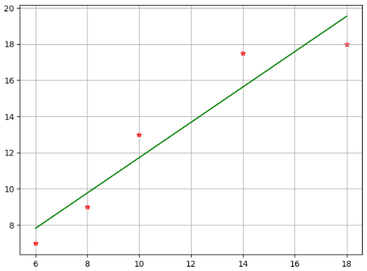
1)一元一次线性方程 y=kx+b
注意x和y一定是[[1],[2],[3],[4],...]
#-*-coding:gb2312-*-
import numpy as np
import matplotlib.pyplot as plt
from sklearn.linear_model import LinearRegression

if __name__ == '__main__':
    x = np.array([6,8,10,14,18])
    y = np.array([7,9,13,17.5,18])
    # 散点图标记为*,颜色为red
    plt.scatter(x,y,marker='*',c='r')
    plt.grid(True)
   # plt.show()

    # 改二维
    # 用数据建立LR模型
#    print(x.reshape(-1,1)) # -1 自动计算
    x_,y_ = x.reshape(-1,1),y.reshape(-1,1)
    lr = LinearRegression() # 截距对结果影响不大
    lr.fit(x_,y_)
    print(lr.intercept_)
    print(lr.coef_) # y = 0.9762931x + 1.96551724

    # 用回归模型预测,颜色用green
    x2 = x
    y2 = lr.predict(x2.reshape(-1,1)).reshape(-1,1)

    plt.plot(x2,y2,'g')
    plt.show()
结果:
2)一元二次方程
输入的x**2和x形式是:[[100,10],[81,9],...]
#-*-coding:gb2312-*-
import numpy as np
import matplotlib.pyplot as plt
from sklearn.linear_model import LinearRegression

if __name__ == '__main__':
    # x = np.array([[10],[9]])
    # print(np.concatenate([x**2,x],axis=1))

    # 设置年份
    year = np.arange(1,12)
    #print(year)
    sale = np.array([0.52,9.36,52,191,350,571,912.17,1207,1682,2135,2684])

    plt.scatter(year,sale,marker="*",c='r')
    plt.grid(True)

    lr = LinearRegression(fit_intercept=False)
    # 重新计算一元二次方程组
    # 输入的x**2和x形式是:[[100,10],[81,9],...]
    x2 = year.reshape(-1,1)
    x2_train = np.concatenate([x2**2,x2],axis=1)
    lr.fit(x2_train,sale.reshape(-1,1))
    print(lr.predict([[144,12]]))

    x3 = x2
    y3 = lr.predict(x2_train).reshape(-1, 1)

    plt.plot(x3, y3, 'g')
    plt.show()
结果:


