机器学习之 KNN近邻算法(二)鸢尾花数据集训练
一、鸢尾花数据集
from sklearn.datasets import load_iris ,通过 datas= load_iris() 获得鸢尾花数据集用于测试
iris里有data和target等等
{'data': array([[5.1, 3.5, 1.4, 0.2],
       [4.9, 3. , 1.4, 0.2],
       [4.7, 3.2, 1.3, 0.2],
       [4.6, 3.1, 1.5, 0.2],
       [5. , 3.6, 1.4, 0.2],
       [5.4, 3.9, 1.7, 0.4],
       [4.6, 3.4, 1.4, 0.3],
       ... 省略 ...
       [6.7, 3. , 5.2, 2.3],
       [6.3, 2.5, 5. , 1.9],
       [6.5, 3. , 5.2, 2. ],
       [6.2, 3.4, 5.4, 2.3],
       [5.9, 3. , 5.1, 1.8]]), 'target': array([0, 0, 0, 0, 0, 0, 0, 0, 0, 0, 0, 0, 0, 0, 0, 0, 0, 0, 0, 0, 0, 0,
       0, 0, 0, 0, 0, 0, 0, 0, 0, 0, 0, 0, 0, 0, 0, 0, 0, 0, 0, 0, 0, 0,
       0, 0, 0, 0, 0, 0, 1, 1, 1, 1, 1, 1, 1, 1, 1, 1, 1, 1, 1, 1, 1, 1,
       1, 1, 1, 1, 1, 1, 1, 1, 1, 1, 1, 1, 1, 1, 1, 1, 1, 1, 1, 1, 1, 1,
       1, 1, 1, 1, 1, 1, 1, 1, 1, 1, 1, 1, 2, 2, 2, 2, 2, 2, 2, 2, 2, 2,
       2, 2, 2, 2, 2, 2, 2, 2, 2, 2, 2, 2, 2, 2, 2, 2, 2, 2, 2, 2, 2, 2,
       2, 2, 2, 2, 2, 2, 2, 2, 2, 2, 2, 2, 2, 2, 2, 2, 2, 2]), 'frame': None, 'target_names': array(['setosa', 'versicolor', 'virginica'], dtype='<U10'), 'DESCR': '.. _iris_dataset:\n\nIris plants dataset\n--------------------\n\n**Data Set Characteristics:**\n\n    :Number of Instances: 150 (50 in each of three classes)\n    :Number of Attributes: 4 numeric, predictive attributes and the class\n    :Attribute Information:\n        - sepal length in cm\n        - sepal width in cm\n        - petal length in cm\n        - petal width in cm\n        - class:\n                - Iris-Setosa\n                - Iris-Versicolour\n                - Iris-Virginica\n                \n    :Summary Statistics:\n\n    ============== ==== ==== ======= ===== ====================\n                    Min  Max   Mean    SD   Class Correlation\n    ============== ==== ==== ======= ===== ====================\n    sepal length:   4.3  7.9   5.84   0.83    0.7826\n    sepal width:    2.0  4.4   3.05   0.43   -0.4194\n    petal length:   1.0  6.9   3.76   1.76    0.9490  (high!)\n    petal width:    0.1  2.5   1.20   0.76    0.9565  (high!)\n    ============== ==== ==== ======= ===== ====================\n\n    :Missing Attribute Values: None\n    :Class Distribution: 33.3% for each of 3 classes.\n    :Creator: R.A. Fisher\n    :Donor: Michael Marshall (MARSHALL%PLU@io.arc.nasa.gov)\n    :Date: July, 1988\n\nThe famous Iris database, first used by Sir R.A. Fisher. The dataset is taken\nfrom Fisher\'s paper. Note that it\'s the same as in R, but not as in the UCI\nMachine Learning Repository, which has two wrong data points.\n\nThis is perhaps the best known database to be found in the\npattern recognition literature.  Fisher\'s paper is a classic in the field and\nis referenced frequently to this day.  (See Duda & Hart, for example.)  The\ndata set contains 3 classes of 50 instances each, where each class refers to a\ntype of iris plant.  One class is linearly separable from the other 2; the\nlatter are NOT linearly separable from each other.\n\n.. topic:: References\n\n   - Fisher, R.A. "The use of multiple measurements in taxonomic problems"\n     Annual Eugenics, 7, Part II, 179-188 (1936); also in "Contributions to\n     Mathematical Statistics" (John Wiley, NY, 1950).\n   - Duda, R.O., & Hart, P.E. (1973) Pattern Classification and Scene Analysis.\n     (Q327.D83) John Wiley & Sons.  ISBN 0-471-22361-1.  See page 218.\n   - Dasarathy, B.V. (1980) "Nosing Around the Neighborhood: A New System\n     Structure and Classification Rule for Recognition in Partially Exposed\n     Environments".  IEEE Transactions on Pattern Analysis and Machine\n     Intelligence, Vol. PAMI-2, No. 1, 67-71.\n   - Gates, G.W. (1972) "The Reduced Nearest Neighbor Rule".  IEEE Transactions\n     on Information Theory, May 1972, 431-433.\n   - See also: 1988 MLC Proceedings, 54-64.  Cheeseman et al"s AUTOCLASS II\n     conceptual clustering system finds 3 classes in the data.\n   - Many, many more ...', 'feature_names': ['sepal length (cm)', 'sepal width (cm)', 'petal length (cm)', 'petal width (cm)'], 'filename': 'D:\\PyProjects\\demo\\venv\\lib\\site-packages\\sklearn\\datasets\\data\\iris.csv'}
二、问题:如何建立最准确的模型?
Question1. 如何科学分配 (train,test) ,按照下标二八分有问题
- Answer1-1: 打乱下标
   # 准备一个乱数的下标序列号
    index=np.arange(150);  # 0~149
    np.random.shuffle(index) # shuffle
   # 根据给定的乱序的下标到对应的数组中提取对应的数据
    train,test=datas.data[index[:100]],datas.data[index[100:]]
    train_target,real_target=datas.target[index[:100]],datas.target[index[100:]]
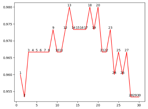
Question2. 如何确定 n_neighbors ?
- Answer2-1:使用 交叉验证方法
为什么要用?
- 最重要:评估模型性能
- Answer1-1的打乱下标方法可以再优化 => 1)交叉验证,相当于扩充了有限数据集;2)用不同数据集测试,可以说明有一定泛化能力
- 确定近邻数n(通过寻找最高的准确率score)=> 求超参数
怎么做?
(设cv=10)所有数据集分成10折,可以保证每折数据集都作为train(9次)和test(1次),最后取mean
相关文章链接1:https://blog.csdn.net/weixin_42211626/article/details/100064842
相关文章链接2:https://blog.csdn.net/qq_36523839/article/details/80707678
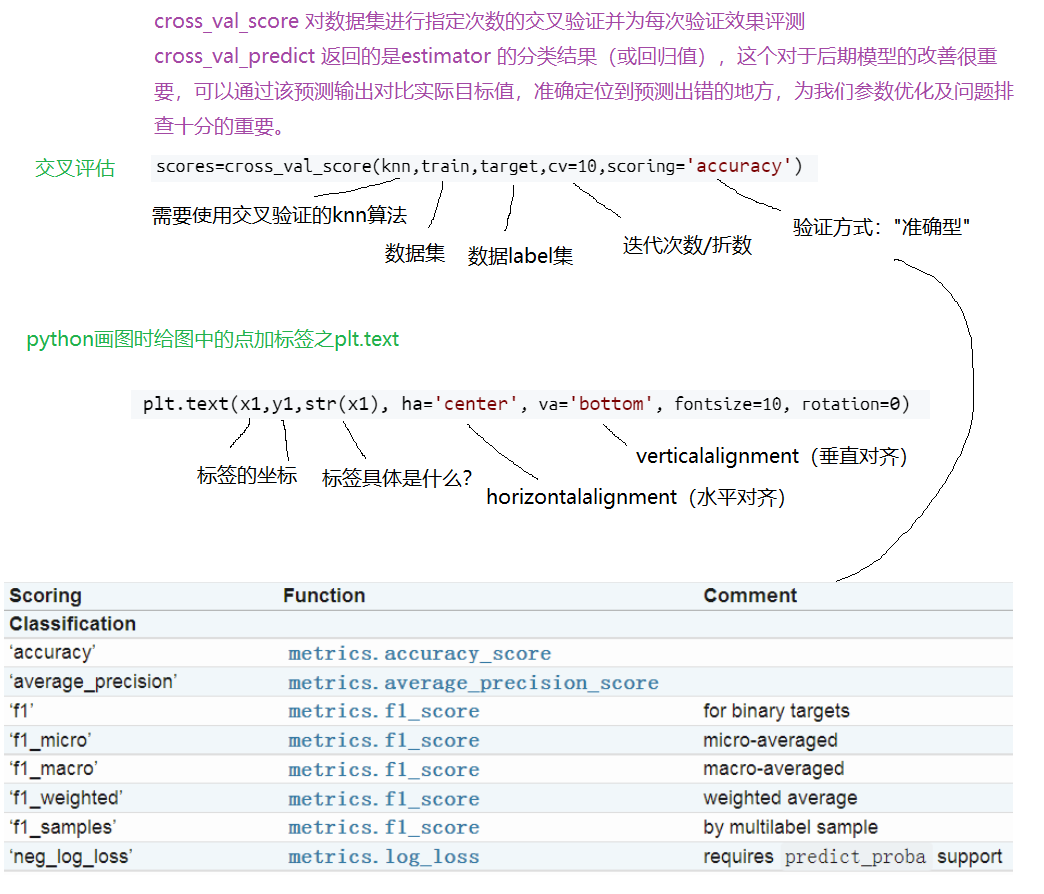
from sklearn.model_selection import cross_val_score
    k_range=range(1,31)
    k_score=[]
    for k in k_range:
        knn=KNeighborsClassifier(n_neighbors=k)
    # 模型评估数据(交叉评估)
    # from sklearn.model_selection import cross_val_score
        scores=cross_val_score(knn,train,target,cv=10,scoring='accuracy')
        k_score.append(scores.mean())
    plt.plot(k_range,k_score,'r')
  # import matplotlib.pyplot as plt
  # plt.text:贴标签
    for x1,y1 in zip(k_range,k_score):
        plt.text(x1,y1,str(x1), ha='center', va='bottom', fontsize=10, rotation=0)
    # 数据作图
   plt.show()
分析:
三、结果