多变量回归

1. 多元特征

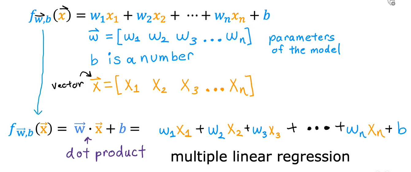
这种具有多个输入特征的线性回归模型被称为，多元线性回归

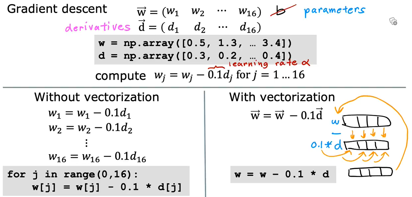
2. 向量化及Numpy

numpy官方说明链接
NumPy 是一个库，它扩展了 python 的基本功能，增加了更丰富的数据集，包括更多数字类型、向量、矩阵和许多矩阵函数。NumPy 和 python 可以无缝协作。Python 算术运算符可用于 NumPy 数据类型，许多 NumPy 函数也可接受 Python 数据类型。NumPy 的基本数据结构是一个可索引的 n 维数组，其中包含相同类型（dtype）的元素。

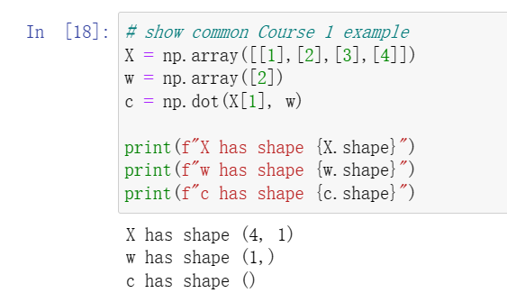
• 关于shape

• 关于reshape

a = np.arange(6).reshape(3, 2) 

重塑命令将a变为 3 行 2 列数组。
参数-1 会告诉例程根据数组的大小和列数计算行数，例如：

Numpy中的dot函数，是两个向量点乘运算的向量化实现
当我们要运算\(f = w_1x_1 + w_2x_2 + ... + w_nx_n\)时，我们可以这样写

import numpy as np
w = np.array([1.0,2.5,-3.3])
b = 4
x = np.array([10,20,30])

f = 0
for i in range(w.shape[0]):
  f += w[i]*x[i]
f += b

利用dot函数，可以这样写

f = np.dot(w , x) + b

不仅更加简单，而且运算效率会更高
也可以与数字相乘

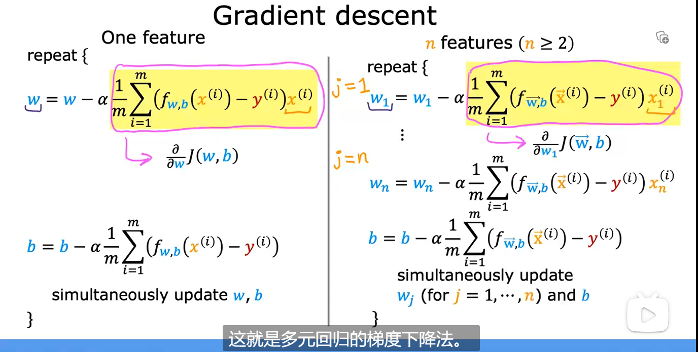
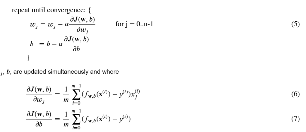
3. 多元线性回归的梯度下降

\[f_{w,b}(x^{(i)}) = w · x^{(i)} + b\\\\ J(w,b) = \frac{1}{2m} \sum_{i = 0}^{m - 1}(f_{w,b}(x^{(i)}) - y^{(i)})^2 \]

计算上述两式：

def compute_cost(X, y, w, b): 
    """
    compute cost
    Args:
      X (ndarray (m,n)): Data, m examples with n features
      y (ndarray (m,)) : target values
      w (ndarray (n,)) : model parameters  
      b (scalar)       : model parameter
      
    Returns:
      cost (scalar): cost
    """
    m = X.shape[0]
    cost = 0.0
    for i in range(m):                                
        f_wb_i = np.dot(X[i], w) + b           #(n,)(n,) = scalar (see np.dot)
        cost = cost + (f_wb_i - y[i])**2       #scalar
    cost = cost / (2 * m)                      #scalar    
    return cost

cost = compute_cost(X_train, y_train, w_init, b_init)

计算6、7式的：

def compute_gradient(X, y, w, b): 
    """
    Computes the gradient for linear regression 
    Args:
      X (ndarray (m,n)): Data, m examples with n features
      y (ndarray (m,)) : target values
      w (ndarray (n,)) : model parameters  
      b (scalar)       : model parameter
      
    Returns:
      dj_dw (ndarray (n,)): The gradient of the cost w.r.t. the parameters w. 
      dj_db (scalar):       The gradient of the cost w.r.t. the parameter b. 
    """
    m,n = X.shape           #(number of examples, number of features)
    dj_dw = np.zeros((n,))
    dj_db = 0.

    for i in range(m):                             
        err = (np.dot(X[i], w) + b) - y[i]   
        for j in range(n):                         
            dj_dw[j] = dj_dw[j] + err * X[i, j]    
        dj_db = dj_db + err                        
    dj_dw = dj_dw / m                                
    dj_db = dj_db / m                                
        
    return dj_db, dj_dw

tmp_dj_db, tmp_dj_dw = compute_gradient(X_train, y_train, w_init, b_init)

计算5式：

def gradient_descent(X, y, w_in, b_in, cost_function, gradient_function, alpha, num_iters): 
    """
    Performs batch gradient descent to learn w and b. Updates w and b by taking 
    num_iters gradient steps with learning rate alpha
    
    Args:
      X (ndarray (m,n))   : Data, m examples with n features
      y (ndarray (m,))    : target values
      w_in (ndarray (n,)) : initial model parameters  
      b_in (scalar)       : initial model parameter
      cost_function       : function to compute cost
      gradient_function   : function to compute the gradient
      alpha (float)       : Learning rate
      num_iters (int)     : number of iterations to run gradient descent
      
    Returns:
      w (ndarray (n,)) : Updated values of parameters 
      b (scalar)       : Updated value of parameter 
      """
    
    # An array to store cost J and w's at each iteration primarily for graphing later
    J_history = []
    w = copy.deepcopy(w_in)  #avoid modifying global w within function
    b = b_in
    
    for i in range(num_iters):

        # Calculate the gradient and update the parameters
        dj_db,dj_dw = gradient_function(X, y, w, b)   ##None

        # Update Parameters using w, b, alpha and gradient
        w = w - alpha * dj_dw               ##None
        b = b - alpha * dj_db               ##None
      
        # Save cost J at each iteration
        if i<100000:      # prevent resource exhaustion 
            J_history.append( cost_function(X, y, w, b))

        # Print cost every at intervals 10 times or as many iterations if < 10
        if i% math.ceil(num_iters / 10) == 0:
            print(f"Iteration {i:4d}: Cost {J_history[-1]:8.2f}   ")
        
    return w, b, J_history #return final w,b and J history for graphing

测试：

# initialize parameters
initial_w = np.zeros_like(w_init)
initial_b = 0.
# some gradient descent settings
iterations = 1000
alpha = 5.0e-7
# run gradient descent 
w_final, b_final, J_hist = gradient_descent(X_train, y_train, initial_w, initial_b,
                                                    compute_cost, compute_gradient, 
                                                    alpha, iterations)
print(f"b,w found by gradient descent: {b_final:0.2f},{w_final} ")
m,_ = X_train.shape
for i in range(m):
    print(f"prediction: {np.dot(X_train[i], w_final) + b_final:0.2f}, target value: {y_train[i]}")

# plot cost versus iteration  
fig, (ax1, ax2) = plt.subplots(1, 2, constrained_layout=True, figsize=(12, 4))
ax1.plot(J_hist)
ax2.plot(100 + np.arange(len(J_hist[100:])), J_hist[100:])
ax1.set_title("Cost vs. iteration");  ax2.set_title("Cost vs. iteration (tail)")
ax1.set_ylabel('Cost')             ;  ax2.set_ylabel('Cost') 
ax1.set_xlabel('iteration step')   ;  ax2.set_xlabel('iteration step') 
plt.show()

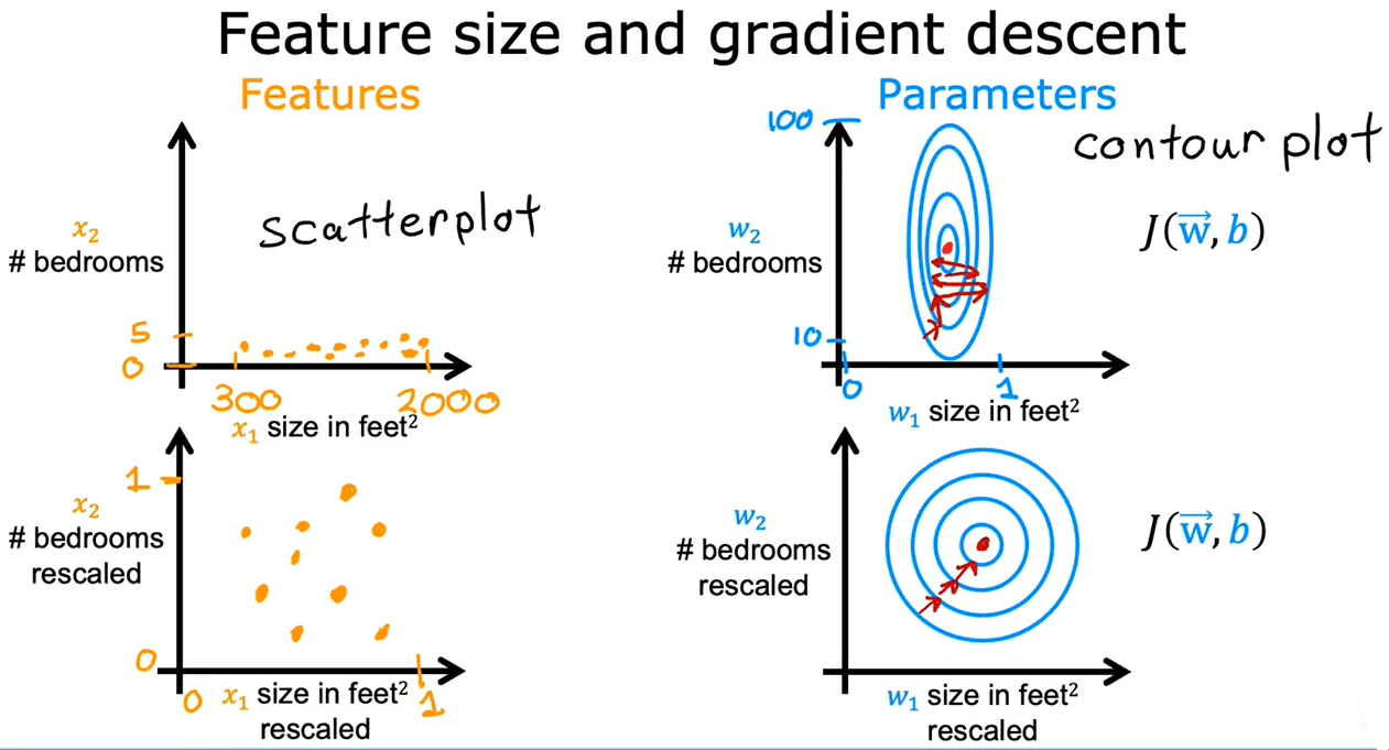
4. 特征放缩

当有不同的特征，且取值差异较大，可能导致梯度下降运行缓慢。通过重新放缩这些特征，使它们都具有可比较的值范围，可显著加快梯度下降速度

特征放缩通常需要将变量放缩至-1~1的区间

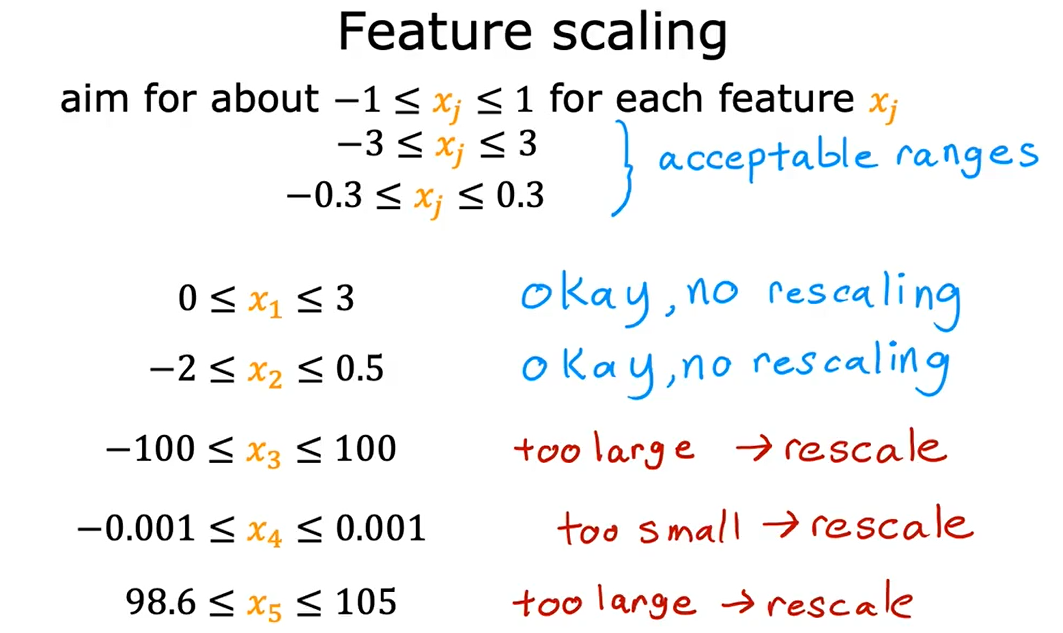
4.1 区间放缩

\[x\prime = \frac{x}{max(x)} \]

若都为正数，取值范围最终为[0,1]。若有正有负，分母就取\(max(abs(x))\),取值范围最终为[-1,1]

4.2 均值归一化

\[x\prime = \frac{x - \overline{x}}{max(x)-min(x)} \]

取值范围最终为[-1 , 1]

4.3 Z-score标准化

\[x\prime = \frac{x - \mu}{\sigma} \]

取值范围最终为正态分布

5. 检查梯度下降是否收敛

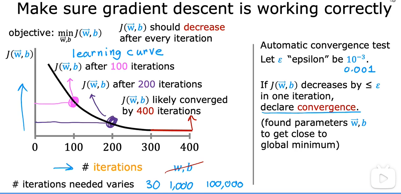
可以画一张左边这样的图，也可以使用右边的自动收敛测试，但是老师倾向于左边

6. 学习率的选择

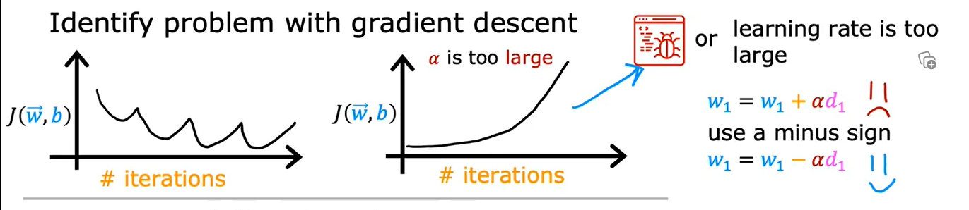
如果J反复横跳或者逐渐变大，说明代码出现了bug或者学习率设置过大
检查方法是把学习率设置为一个非常非常小的数，再跑一遍，如果还出现上述情况，就是代码有bug，例如将\(w = w - \alpha d\)写成了+

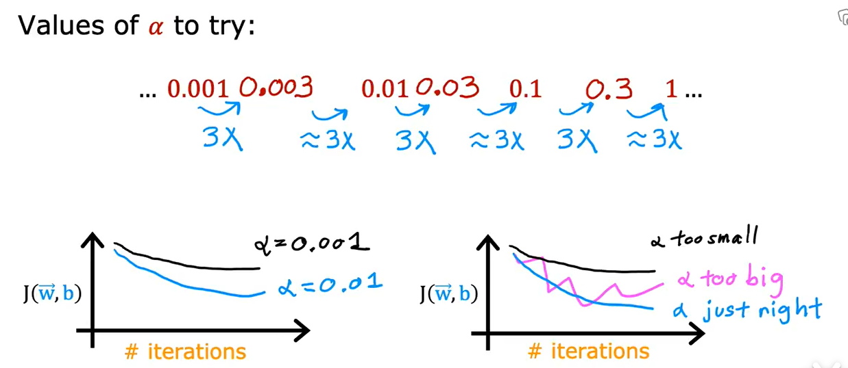
可以先设为0.001，再逐渐增加为上一次3倍的学习率并绘制迭代此处-代价函数图像，直到找到合适学习率

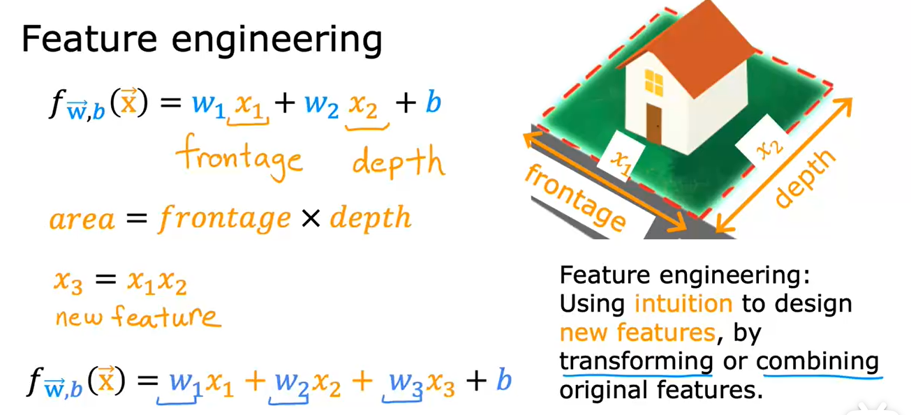
7. 特征工程

运用你的直觉或者知识去设计新的特征，通过合并或变换原有的问题特征，使其能帮助算法更简单地做出准确预测。
这取决于你对实际工程应用的理解