

Real estate analysis report - data from Lianjia.com
Final work for lianjia data analysis
Ningzhi Wang
2023-01-13
This is the final data analysis report of Real-estate from Lianjia.com. Documented by Ningzhi Wang.
# pre-porcessing
lj$age <- 2019 - lj$building_year
lj$price_sqm_k <- lj$price_sqm/1000
lj$price_ttl_m <- lj$price_ttl/1000000
pattern <- "(?<line>[0-9]+)"
result <- regexpr(pattern= pattern, text = lj$line, perl=TRUE)
start <- attr(result,"capture.start")
length <- attr(result,"capture.length")
name <- attr(result,"capture.name")
lj$newline <- ifelse(start > 0,
                     substr(lj$line, start[,name],start[,name] + length[,name]-1),NA)
length <- attr(result,"capture.length")
name <- attr(result,"capture.name")
lj$newline <- ifelse(start > 0,
                     substr(lj$line, start[,name],start[,name] + length[,name]-1),NA)

lj$height <- lj$building_height
lj$area <- lj$building_area
Variables definition numeric: 1. price_sqm_k (price pre square meter, unit: thousand RMB) 2. price_ttl (total price, unit: 10k RMB) 2. age (years between 2019 and build date) 3. building_height (the height of the building, unit: meters) 4. bedrooms (number of bedrooms) 5. has_elevator (0 denotes haven’t elevator, 1 otherwise)
factors: 1. hml (higher floor, middle floor, lower floor) 2. station (denotes the name of the nearest railway station) 3. building_location (denotes the approximate location of the building)
1 Discriptive statistics
There are 6286 observations in the dataset. The mean price sqm is 67.76k RMB, the mean total price is 6.03 million, the mean age is 23 years, the mean building height is 12.76 meters. The average number of bedrooms is approximately 2, 45% of the houses have elevators.
Table 1 Discriptive statistics
lj %>%
  # remove duplications
  unique() %>%
  # select numeric variables
  select(price_sqm_k,price_ttl,age,building_height,bedrooms,has_elevator) %>%
  # show discription
  describe()
2 Single variable analysis
2.1 price hist
The price sqm is approximatly normally distributed, with a median of 64126 RMB.
p<- lj %>%
ggplot() +
geom_histogram(aes(price_sqm),col="white",fill="lightskyblue")
p +
labs(title = "Figure 1.1: Histogram of Price per square meter",
subtitle = "in RMB",
caption = "(Source: Lianjia, Shanghai)",
x = "Price/Square",
y = "Counts") +
theme(plot.title = element_text(size = 15,
hjust = 0.5,
vjust = 0.5,
angle = 0,
),
plot.subtitle = element_text(hjust = 0),
plot.caption = element_text(vjust = 0.5,hjust = 0.5,color = 'darkgreen')) +
geom_vline(aes(xintercept = median(price_sqm)),color='red',linetype="dashed") +
geom_text(aes(x = median(price_sqm)+12000,y=-10,label = median(price_sqm)),color='red',size = 2)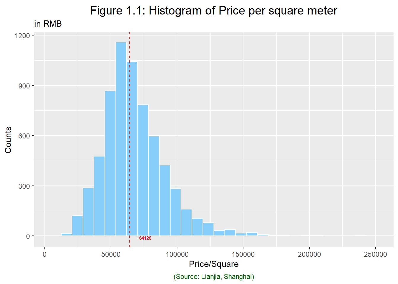 The total price presents a serious right deviation distribution, but most of the observations are consentrated around the median. The median ttl is 4.3 million RMB.
#### price hist
p<- lj %>%
    ggplot() +
    geom_histogram(aes(price_ttl),col="white",fill="lightskyblue")
p +
  labs(title = "Figure 1.2: Histogram of Total Price",
       subtitle = "in 10k RMB",
       caption = "(Source: Lianjia, Shanghai)",
       x = "Total Price",
       y = "Counts") +
  theme(plot.title = element_text(size = 15,
                                  hjust = 0.5,
                                  vjust = 0.5,
                                  angle = 0,
                                  ),
        plot.subtitle = element_text(hjust = 0),
        plot.caption = element_text(vjust = 0.5,hjust = 0.5,color = 'darkgreen')) +
  geom_vline(aes(xintercept = median(price_ttl)),color='red',linetype="dashed") +
  geom_text(aes(x = median(price_ttl),y=-10,label = median(price_ttl)),color='red',size = 2)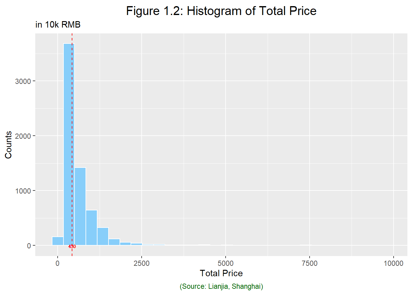
2.2 Building Age
The median age of the buildings is 23 years, with a few outliers have the age of more than 60 years and even 90 years.
p<- lj %>%
    ggplot() +
    geom_histogram(aes(age),col="white",fill="lightskyblue")
p +
  labs(title = "Figure 2: Histogram of building age",
       subtitle = "in YEAR",
       caption = "(Source: Lianjia, Shanghai)",
       x = "Year",
       y = "Counts")+
  theme(plot.title = element_text(size = 15,
                                  hjust = 0.5,
                                  vjust = 0.5,
                                  angle = 0,
  ),
  plot.subtitle = element_text(hjust = 0),
  plot.caption = element_text(vjust = 0.5,hjust = 0.5,color = 'darkgreen')) +
  geom_vline(aes(xintercept = median(age)),color='red',linetype="dashed") +
  geom_text(aes(x = median(age)+2,y=-10,label = median(age)),color='red',size = 2)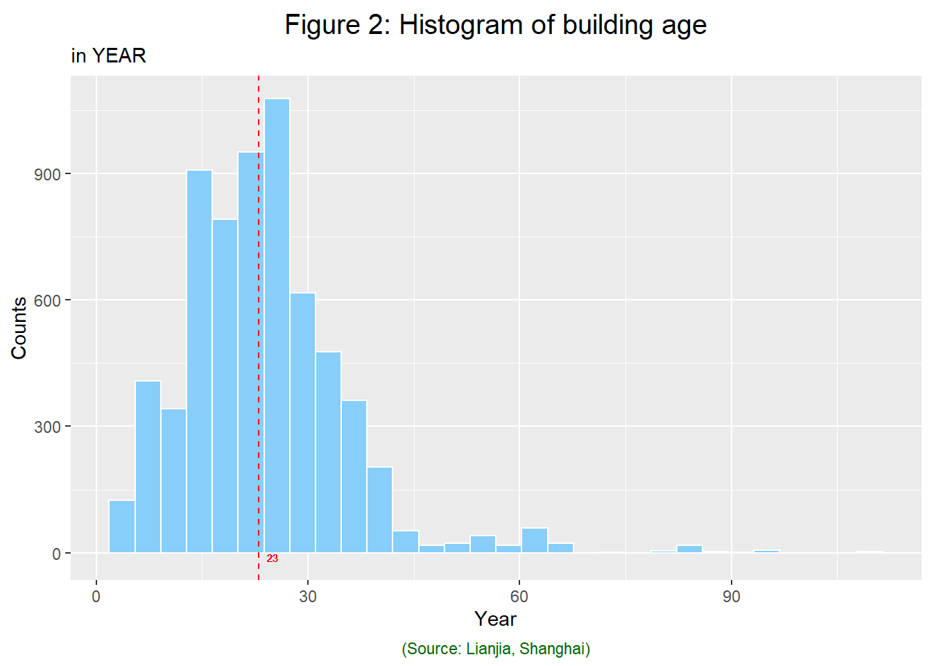
2.3 The Number of Bedrooms
Most of the observations, have less than 3 bedrooms.
lj %>%
mutate(bedrooms = as.factor(bedrooms)) %>%
count(bedrooms) %>%
ggplot(aes(x = reorder(bedrooms,-n), n)) +
geom_bar(stat="identity",col="white",fill="lightskyblue") +
geom_text(aes(label = n),vjust=-0.5) +
labs(title = "Figure 3: Histogram of Bedrooms",
caption = "(Source: Lianjia, Shanghai)",
x = "Number of Bedrooms",
y = "Counts")+
theme(plot.title = element_text(size = 15,
hjust = 0.5,
vjust = 0.5,
angle = 0,
),
plot.caption = element_text(vjust = 0.5,hjust = 0.5,color = 'darkgreen'))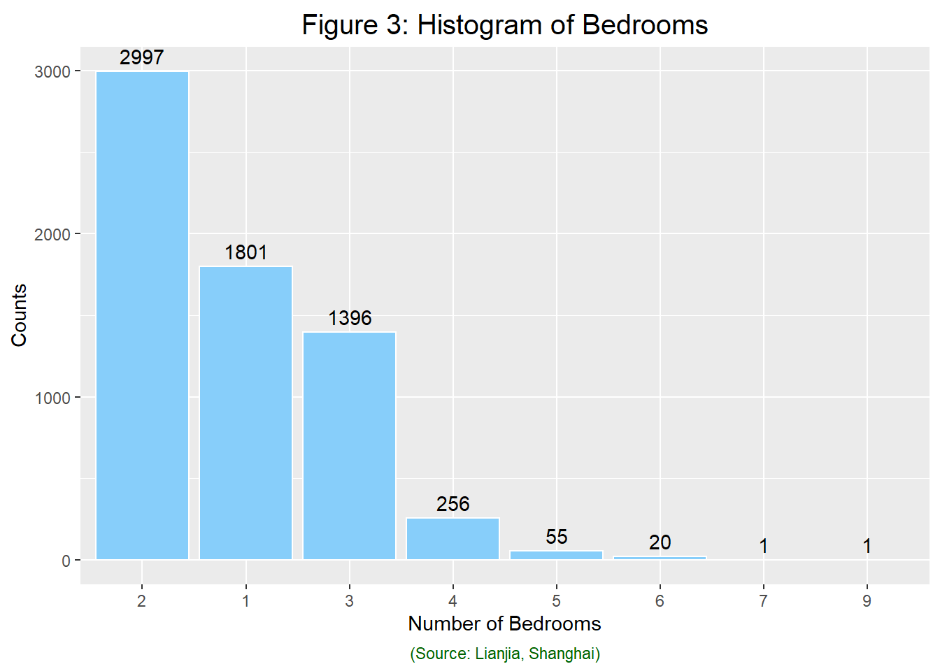 #### 2.4 Building Height A large number of observations are of the height of 7 meters, while the others are relatively uniformly distributed between 3 and 40 meters. This might due to problems left over from history, that is, there are still a large number of low-rise houses with small property rights.
p<- lj %>%
    ggplot() +
    geom_histogram(aes(building_height),col="white",fill="lightskyblue")
p +
  labs(title = "Figure 2: Histogram of building height",
       subtitle = "in Meters",
       caption = "(Source: Lianjia, Shanghai)",
       x = "Meter",
       y = "Counts")+
  theme(plot.title = element_text(size = 15,
                                  hjust = 0.5,
                                  vjust = 0.5,
                                  angle = 0,
  ),
  plot.subtitle = element_text(hjust = 0),
  plot.caption = element_text(vjust = 0.5,hjust = 0.5,color = 'darkgreen')) +
  geom_vline(aes(xintercept = median(building_height)),color='red',linetype="dashed") +
  geom_text(aes(x = median(building_height)+2,y=-10,label = median(building_height)),color='red',size = 2)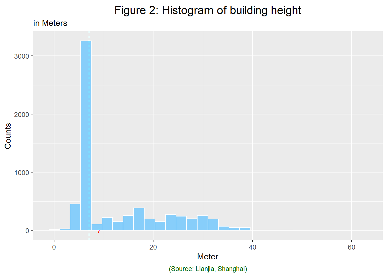
3 Multi Variables
3.1 elevator & bedrooms
An obvious trend is that the more bedrooms an apartment have, the more likely it has elevators. The percentage of having elevators is less than half only for observations with 1 or 2 bedrooms.
nl <- table(lj$has_elevator, lj$bedrooms, dnn = c("has_elevator","bedrooms")) %>%
  prop.table(margin = 2) %>%
  round(2) %>%
  as.data.frame(responseName = "prop") %>%
  arrange(has_elevator, prop) %>%
  filter(has_elevator == 1) %>%
  pull(bedrooms) %>%
  as.character()

lj %>%
  ggplot(aes(x=fct_relevel(factor(bedrooms),nl), fill=factor(has_elevator))) +
  geom_bar(position = "fill") +
  labs(title = "Figure 4: Bedrooms and Elevator",
       caption = "(Source: Lianjia, Shanghai)",
       x = "Bedrooms",
       y = "Have elevator (%)")+
  theme(plot.title = element_text(size = 15,
                                  hjust = 0.5,
                                  vjust = 0.5,
                                  angle = 0,
  ),
  plot.caption = element_text(vjust = 0.5,hjust = 0.5,color = 'darkgreen'))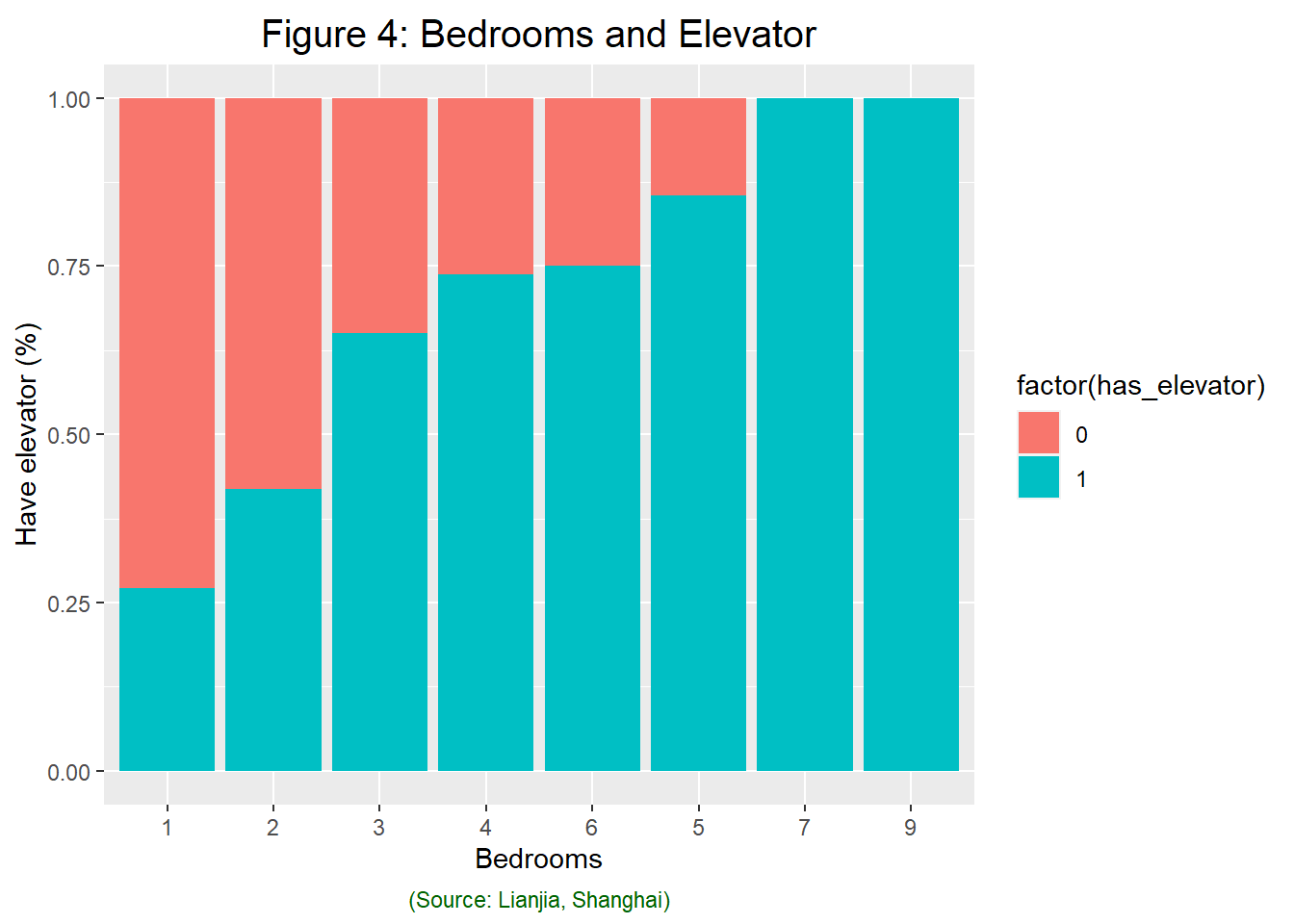
3.2 elevator & lines
The line with the lowest proportion of elevators is the extension section of Line 5, and the line with the highest proportion is the Pujiang Line. Generally speaking, the proportion of suburban houses with elevators is small.
nl <- table(lj$has_elevator, lj$line, dnn = c("has_elevator","line")) %>%
  prop.table(margin = 2) %>%
  round(2) %>%
  as.data.frame(responseName = "prop") %>%
  arrange(has_elevator, prop) %>%
  filter(has_elevator == 1) %>%
  pull(line) %>%
  as.character()
lj %>%
  ggplot(aes(x=fct_relevel(factor(line),nl), fill=factor(has_elevator))) +
  geom_bar(position = "fill") +
  labs(title = "Figure 5: Line and Elevator",
       caption = "(Source: Lianjia, Shanghai)",
       x = "Line",
       y = "Have elevator (%)")+
  theme(plot.title = element_text(size = 15,
                                  hjust = 0.5,
                                  vjust = 0.5,
                                  angle = 0,
  ),
  plot.caption = element_text(vjust = 0.5,hjust = 0.5,color = 'darkgreen'),
  axis.text.x = element_text(angle=30,size = 6,vjust=1,hjust=1))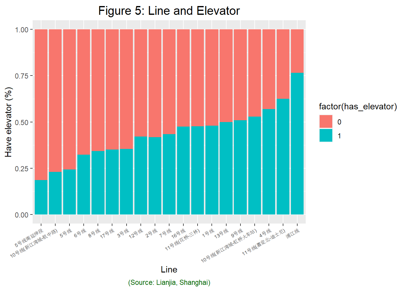
3.3 building area and ttl
Obviously, the larger the building area, the higher the total price of the house. However, this phenomenon is more intuitive in houses below 400 square meters. If you only look at houses over 400 square meters, this positive correlation will obviously weaken or even disappear.
temp <- lj %>%
  filter(building_area > 400)

temp2 <- lj %>%
  filter(building_area>200 & price_ttl < 1000)

p <- ggplot() +
  geom_point(data=lj, aes(x=building_area, y=price_ttl), shape=1,alpha = 0.1) +
  geom_point(data=temp, aes(x=building_area, y=price_ttl),
             color='red',shape=24) +
  geom_point(data = temp2, aes(x=building_area, y=price_ttl),
             color="blue",shape = 21)
p +
  labs(title = "Figure 6: Building area and TTL",
       caption = "(Source: Lianjia, Shanghai)",
       x = "Building area (m2)",
       y = "Price TTL (10k)")+
  theme(plot.title = element_text(size = 15,
                                  hjust = 0.5,
                                  vjust = 0.5,
                                  angle = 0,
  ),
  plot.caption = element_text(vjust = 0.5,hjust = 0.5,color = 'darkgreen'))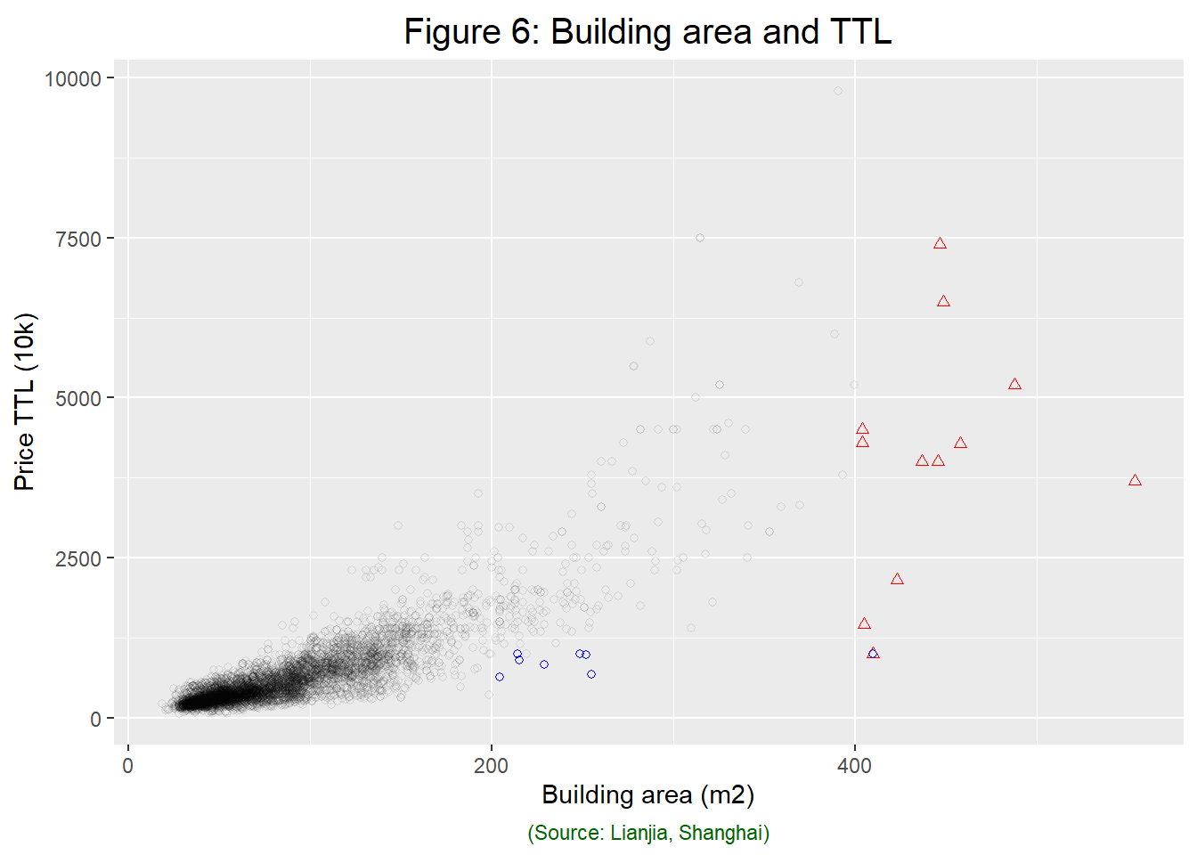
3.4 Building area, TTL, elevators & Line
In all lines, the total price of houses rises with the increase of construction area. In most lines, the increase is steeper in the group with elevators, that is, the square meter price of houses with elevators is higher. However, Line 17, Line 5 and Line 6 are exceptions. The square meter price of groups with and without elevators is similar.
p <- ggplot(lj, aes(x=building_area, y=price_ttl, color = factor(has_elevator))) +
  geom_point(shape=1) +
  geom_smooth(method="lm") +
  facet_wrap( ~ line)+
  coord_cartesian(xlim = c(0,100), ylim=c(0,1000)) +
  theme(text=element_text(size=10))

p +
  labs(title = "Figure 7: Building area, TTL, elevators & Line",
       caption = "(Source: Lianjia, Shanghai)",
       x = "Building area (m2)",
       y = "Price TTL (10k)")+
  theme(plot.title = element_text(size = 15,
                                  hjust = 0.5,
                                  vjust = 0.5,
                                  angle = 0,
  ),
  plot.caption = element_text(vjust = 0.5,hjust = 0.5,color = 'darkgreen'))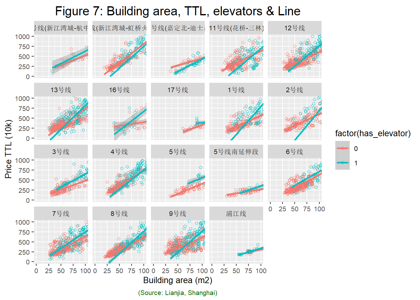
3.5 number of bedrooms & sqm
When the number of bedrooms is less than 5, the more the number of bedrooms, the higher the price of square meters, which also represents the rule of most samples. When the number of bedrooms is 6-7, the price of square meters will gradually decrease. However, when the number of bedrooms is 9, the price per square meter is the highest.
boxplot(lj$price_sqm_k ~ lj$bedrooms,xlab="",ylab="")
title(main = "Figure 8: Bedrooms and SQM", xlab = "Number of bedrooms", ylab = "Price SQM")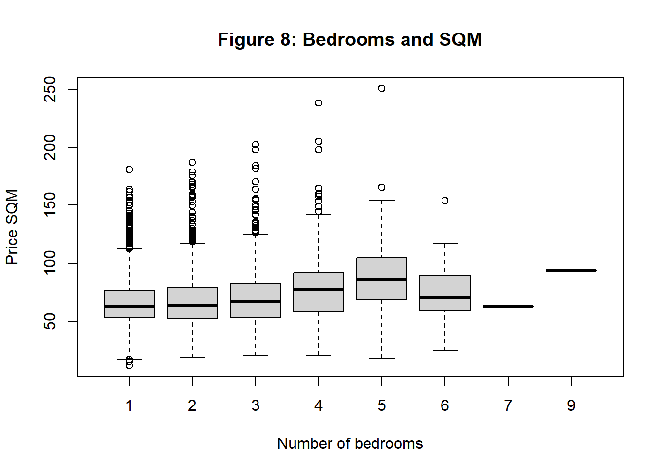
The following figure shows the relationship between the square meter price of the house and the number of rooms. The price of most houses per square meter is less than 100k RMB. When the number of rooms is less than 3, the price per square meter is the most in the range of about 700-800k RMB.
p <-
  lj %>%
  ggplot() +
  geom_freqpoly(aes(price_sqm_k,color=as.factor(bedrooms))) +
  theme(text = element_text(size=12,face="bold"))
p +
  labs(title = "Figure 9: distribution of SQM group by Bedrooms",
       caption = "(Source: Lianjia, Shanghai)",
       x = "Price SQM (k)",
       y = "Counts")+
  theme(plot.title = element_text(size = 15,
                                  hjust = 0.5,
                                  vjust = 0.5,
                                  angle = 0,
  ),
  plot.caption = element_text(vjust = 0.5,hjust = 0.5,color = 'darkgreen'))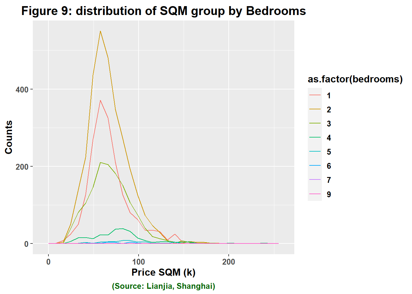
3.6 hml & price
The following figure shows the distribution of the square meter price of houses with different floors in the group with and without elevators.
In most groups, the square meter price of houses is concentrated in the range of 5-7k RMB. However, for the groups without elevators, the price of high-rise buildings tends to be left, that is, the unit price of square meters is lower, while the unit price of square meters of lower floors is higher.
Strangely, in the group without elevators, the number of houses on sale in the high-rise is more, while the number of houses on sale in the lower floors is the least.
p <- lj %>%
filter(hml %in% c("高","中","低")) %>%
ggplot() +
geom_freqpoly(aes(price_sqm_k,color=hml)) +
facet_wrap(~as.factor(has_elevator)) +
theme(text = element_text(size=12,face="bold"))
p +
labs(title = "Figure 10: Price distribution group by Height/elevators",
caption = "(Source: Lianjia, Shanghai)",
x = "Price TTL (10k)",
y = "Counts")+
theme(plot.title = element_text(size = 15,
hjust = 0.5,
vjust = 0.5,
angle = 0,
),
plot.caption = element_text(vjust = 0.5,hjust = 0.5,color = 'darkgreen'))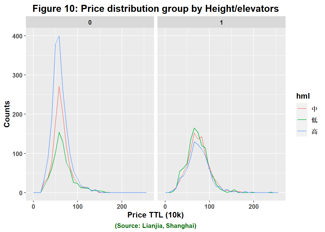 #### 3.7 metro lines & sqm The price of Line 17 and Line 5 is obviously low, which may be due to the main layout in the suburbs.
boxplot(lj$price_sqm_k ~ lj$newline, xlab="Line", ylab="price SQM (k)")
title(main = "Figure 11: Subway Line and price SQM")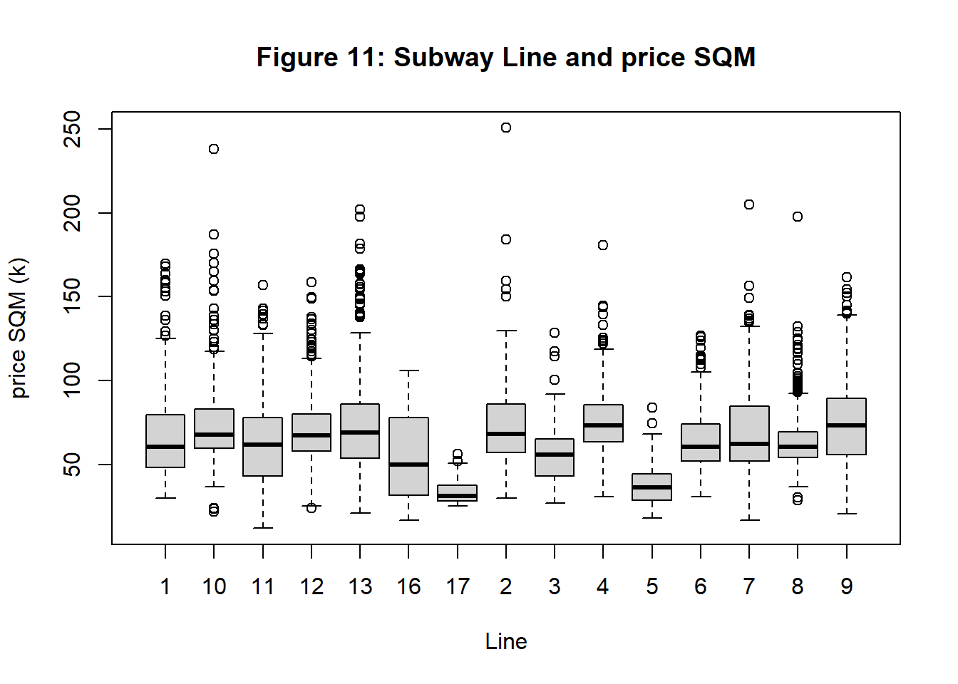
3.8 metro lines & bedrooms
The number of bedrooms on most lines is 2, only 3 for Line 17. This is interesting, because we have just analyzed that the unit price per square meter of Line 17 is the lowest, so the low unit price per square meter of Line 17 is probably due to the larger area.
boxplot(lj$bedrooms ~ lj$newline, xlab="Line", ylab="Bedrooms")
title(main = "Figure 12: Subway Line and Bedrooms")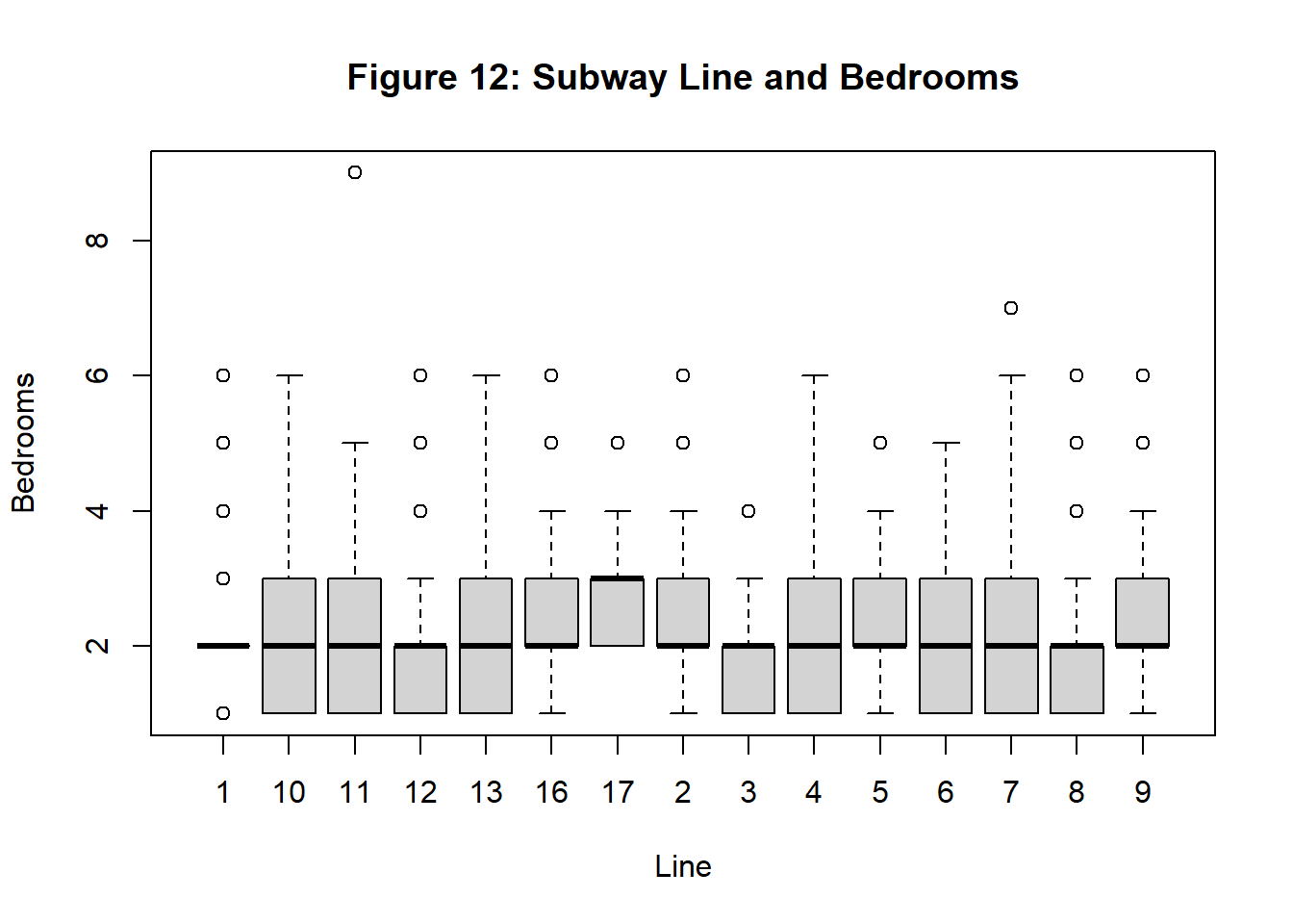
3.9 decoration & elevator & area & price
We will consider the decoration style, elevator and housing area together. As shown in the figure below, the hardbound room has a higher unit price and total price than the simple decoration and blank.
Houses with elevators tend to have larger area (higher position) and higher total price (larger point size). However, in terms of unit price, this picture cannot show the obvious difference between the houses with elevators and without elevators. It can only be roughly reflected in the area with the highest unit price, which is basically the hardbound elevator apartment.
qplot(price_sqm_k,building_area,data = lj, color = factor(has_elevator),shape = factor(decoration), size = price_ttl_m, main = "Figure 13: Area & TTL & Elevator & Decoration", ylab = "Building area (m2)", xlab = "price SQM (k)")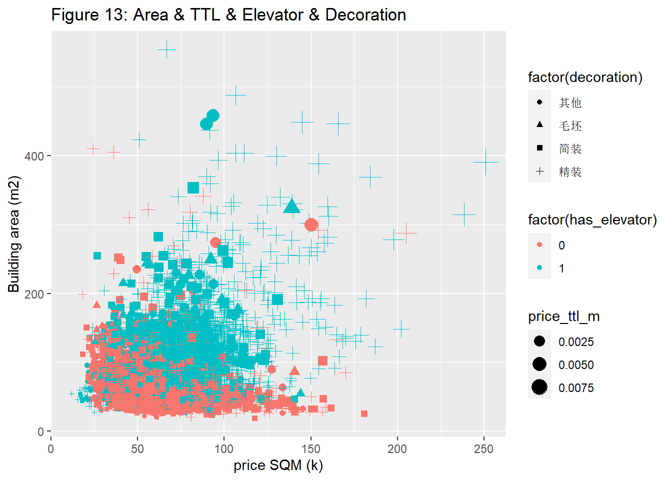 #### 3.10 building height & hml & elevator & price It can be seen from this picture that the houses without elevators will not exceed a certain height (about 8 meters), and the houses with elevators will not be hindered by this. It can’t be seen from this picture that there is a clear relationship between the height of the house and the total price. We can see some high price houses with very low height from the picture, which may be villas. Therefore, the type of the house may also be an important factor affecting the price.
qplot(price_sqm_k,building_height,data = lj, color = factor(has_elevator),shape = factor(decoration), size = price_ttl_m, main = "Figure 13: Height & TTL & Elevator & Decoration", ylab = "Building height (m)", xlab = "price SQM (k)")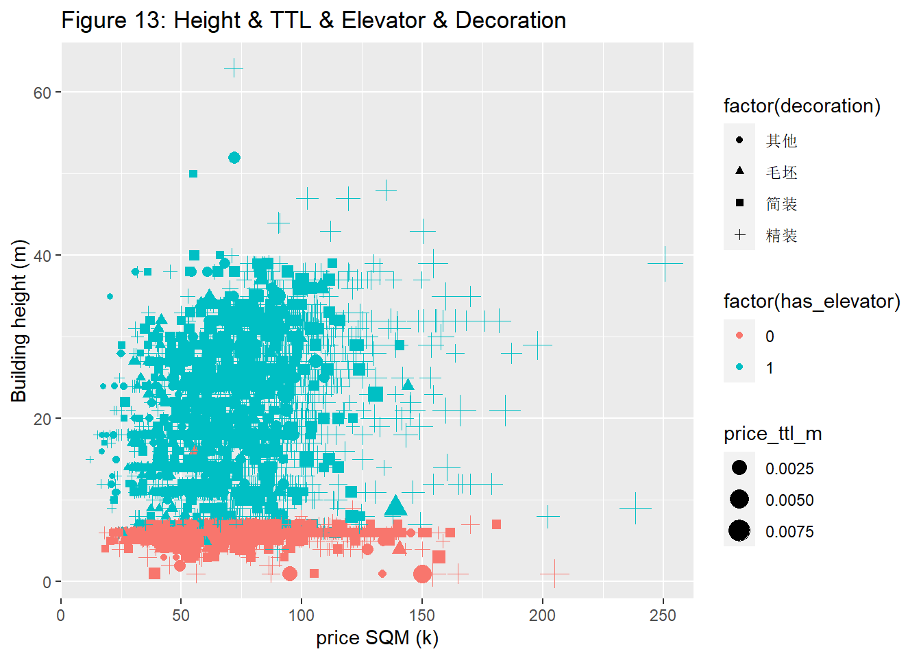
3.11 numbers based on line
Line 8 has the largest number of houses on sale, close to 800 sets. Line 17 is the least, less than 50 sets.
temp <- count(lj,line)

p <-
  temp %>%
  ggplot() +
  geom_col(aes(x = reorder(line,-n),y=n),fill = "lightskyblue",alpha = 0.5) +
  theme(axis.text.x = element_text(angle=30,size = 6,vjust=1,hjust=1))

p +
  labs(title = "Figure 14: Count across lines",
       caption = "(Source: Lianjia, Shanghai)",
       x = "Line",
       y = "Counts")+
  theme(plot.title = element_text(size = 15,
                                  hjust = 0.5,
                                  vjust = 0.5,
                                  angle = 0,
  ),
  plot.caption = element_text(vjust = 0.5,hjust = 0.5,color = 'darkgreen'))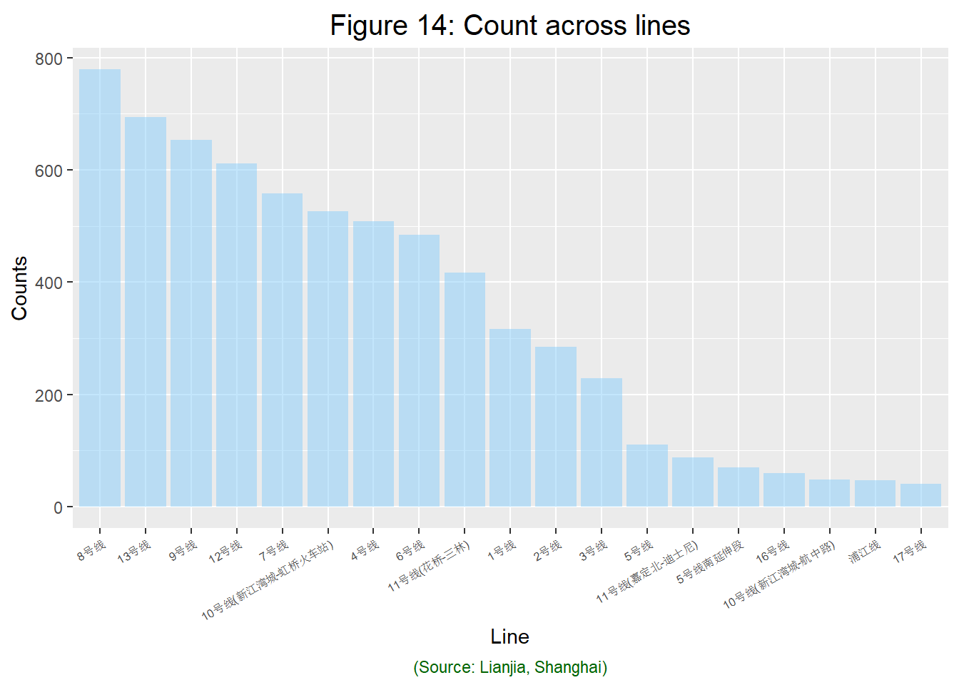
3.12 price across lines
Next, we will divide the price into five sections, and then analyze the percentage of house prices on different subway lines in these five sections. Obviously, the houses on Line 17, Line 11, Line 5 and Pujiang Line are generally low. The distribution of housing prices on other lines is relatively uniform. This reminds us again that location is very important for house pricing.
lj <- mutate(lj,price_sqm_hl = cut(price_sqm,
                                   quantile(price_sqm,
                                            probs = seq(0,1,length.out = 6)),
                                   labels = c("lowest","below average","average","higher than average","highest"),
                                   include.lowest = TRUE))

ggplot(lj,aes(x = line,fill=price_sqm_hl)) +
  geom_bar(position = "fill") +
  scale_fill_brewer("price", type="div", palette="PiYG") +
  labs(title = "Figure 15: Line and Price SQM",
       caption = "(Source: Lianjia, Shanghai)",
       x = "Line",
       y = "Price SQM (%)")+
  theme(plot.title = element_text(size = 15,
                                  hjust = 0.5,
                                  vjust = 0.5,
                                  angle = 0,
  ),
  plot.caption = element_text(vjust = 0.5,hjust = 0.5,color = 'darkgreen'),
  axis.text.x = element_text(angle=30,size = 6,vjust=1,hjust=1))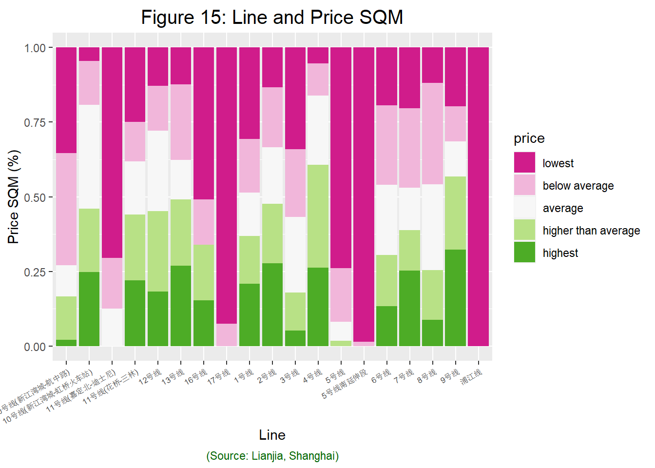
4 Econometric Model
The square meter price of hardcover is the highest, followed by simple decoration, and then the blank and others. At the same time, the rate of elevator and the height of the house are the highest. But the housing age of the blank is the lowest. ##### Table 3 summary stats group by decoration
library(plotly)##
## 载入程辑包:'plotly'## The following object is masked from 'package:ggplot2':
##
## last_plot## The following object is masked from 'package:stats':
##
## filter## The following object is masked from 'package:graphics':
##
## layoutlj$area <- lj$building_area
lj$height <- lj$building_height
newlj <- lj[,c('decoration','price_sqm','price_ttl','bedrooms','has_elevator','height','age','area')]
newlj %>%
group_by(decoration) %>%
group_modify(~{
.x %>%
purrr::map_dfc(mean, na.rm = TRUE)
}) %>% ungroup() Table 4 Difference test for Blank and simple decoration
Because simple decoration has disadvantages in terms of age, elevator and number of bedrooms, although the average unit price is higher, we still need to further analyze whether there are actual differences between simple decoration and rough decoration. The following table shows that the blank is significantly lower than the simple SQM, but the total price not statistically significant. Nevertheless, the difference between simple decoration and blank is significant in most variables, indicating that there are systematic differences between the two groups, not just decoration.
newlj %>%
  filter(decoration %in% c("毛坯","简装")) %>%
  pivot_longer(cols = -decoration, names_to = "variable", values_to = "value") %>%
  group_nest(variable) %>%
  mutate(t.test = map(data, ~ tidy(t.test(value ~ decoration, data = .x)))) %>%
  unnest(t.test) %>%
  select(-data)
Table 5 Difference test for Hardbound and simple decoration
The roughcast room is younger than the hardbound room, but the number of elevators is less, but the difference is not significant. The number of space and bedrooms in the roughcast room is less, the floor is lower, and the total price and unit price are lower. It can be speculated that the investment purpose of rough housing is more obvious.
newlj %>%
  filter(decoration %in% c("毛坯","精装")) %>%
  pivot_longer(cols = -decoration, names_to = "variable", values_to = "value") %>%
  group_nest(variable) %>%
  mutate(t.test = map(data, ~ tidy(t.test(value ~ decoration, data = .x)))) %>%
  unnest(t.test) %>%
  select(-data)
Table 6 Difference test of floor height
newlj <- lj[,c('hml','price_sqm','price_ttl','bedrooms','has_elevator','height','age','area')]
newlj %>%
  filter(hml %in% c("高","低")) %>%
  pivot_longer(cols = -hml, names_to = "variable", values_to = "value") %>%
  group_nest(variable) %>%
  mutate(t.test = map(data, ~ tidy(t.test(value ~ hml, data = .x)))) %>%
  unnest(t.test) %>%
  select(-data)
Table 7 Regression model1
The housing area, housing year and housing height are significantly related to the price. The price of the square meter will increase by 59 RMB for every square meter of the house area. The price of the square meter will increase by 625 RMB for each year the age of the house increases. The price of the square meter will increase by 959 RMB for every 1 meter increase in the height of the house. Having elevator will increase SQM by 3887 RMB. The price of slab building is 11784 RMB higher than that of tower building. At present, the R square of the model is only 0.21.
smodel <- lm(price_sqm ~ decoration + building_area + age + building_height + building_style + has_elevator, data = lj)
summary(smodel)##
## Call:
## lm(formula = price_sqm ~ decoration + building_area + age + building_height +
## building_style + has_elevator, data = lj)
##
## Residuals:
## Min 1Q Median 3Q Max
## -69482 -12731 -2312 10208 158973
##
## Coefficients:
## Estimate Std. Error t value Pr(>|t|)
## (Intercept) 17297.748 1719.064 10.062 < 2e-16 ***
## decoration毛坯 -3046.074 1626.208 -1.873 0.06110 .
## decoration简装 3496.733 1111.306 3.147 0.00166 **
## decoration精装 11060.496 1097.591 10.077 < 2e-16 ***
## building_area 59.349 6.353 9.342 < 2e-16 ***
## age 625.533 27.582 22.679 < 2e-16 ***
## building_height 959.335 48.862 19.633 < 2e-16 ***
## building_style板塔结合 2229.049 3817.608 0.584 0.55932
## building_style板楼 11783.503 887.616 13.275 < 2e-16 ***
## has_elevator 3887.464 975.884 3.984 6.86e-05 ***
## ---
## Signif. codes: 0 '***' 0.001 '**' 0.01 '*' 0.05 '.' 0.1 ' ' 1
##
## Residual standard error: 20910 on 6517 degrees of freedom
## Multiple R-squared: 0.2186, Adjusted R-squared: 0.2175
## F-statistic: 202.6 on 9 and 6517 DF, p-value: < 2.2e-16Table 8 Regression model2
Adding direction factor does little to increase R square.
smodel <- lm(price_sqm ~ decoration + building_area + age + building_height + building_style + has_elevator + directions1, data = lj)
summary(smodel)##
## Call:
## lm(formula = price_sqm ~ decoration + building_area + age + building_height +
## building_style + has_elevator + directions1, data = lj)
##
## Residuals:
## Min 1Q Median 3Q Max
## -71135 -12800 -2356 10243 159099
##
## Coefficients:
## Estimate Std. Error t value Pr(>|t|)
## (Intercept) 19100.484 2293.957 8.326 < 2e-16 ***
## decoration毛坯 -3159.947 1627.550 -1.942 0.05224 .
## decoration简装 3402.419 1112.908 3.057 0.00224 **
## decoration精装 11010.689 1098.645 10.022 < 2e-16 ***
## building_area 58.559 6.378 9.181 < 2e-16 ***
## age 626.835 27.680 22.646 < 2e-16 ***
## building_height 960.639 49.059 19.581 < 2e-16 ***
## building_style板塔结合 1830.228 3823.178 0.479 0.63215
## building_style板楼 11748.499 923.142 12.727 < 2e-16 ***
## has_elevator 3914.002 977.196 4.005 6.26e-05 ***
## directions1东北 4964.305 4551.641 1.091 0.27546
## directions1东南 -2713.642 2033.799 -1.334 0.18216
## directions1北 -3922.270 2431.405 -1.613 0.10676
## directions1南 -1651.089 1628.505 -1.014 0.31068
## directions1暂无数据 -3935.610 3079.261 -1.278 0.20126
## directions1西 -6753.541 2885.790 -2.340 0.01930 *
## directions1西北 5756.020 3628.808 1.586 0.11274
## directions1西南 -1369.858 2254.472 -0.608 0.54346
## ---
## Signif. codes: 0 '***' 0.001 '**' 0.01 '*' 0.05 '.' 0.1 ' ' 1
##
## Residual standard error: 20900 on 6509 degrees of freedom
## Multiple R-squared: 0.2205, Adjusted R-squared: 0.2185
## F-statistic: 108.3 on 17 and 6509 DF, p-value: < 2.2e-16Table 9 Regression model2
In order to increase the explanatory power of the model, we have added decoration, orientation and location. At this time, the coefficient of house age is completely reversed, the house age increases by 1 year, and the square meter price decreases by 166 yuan.
When the height increase by 1m, price SQM will increase by 14 yuan, which is economically and statistically not significant.
The coefficient of the building area is still positive, with an increase of 1 square meter and an increase of 45 yuan per square meter. Meaning that smaller house is generally more cost effective.
The coefficients of building_style remain robust, The price of slab building is 10090 RMB higher than that of tower building.
In addition, the hardbound houses are 2192 yuan per square meter more expensive than the category “others”, and the price of simple decoration and rough decoration is lower than that of “other” square meters.
Another obvious phenomenon is that location plays a key role in improving the interpretation of the model. The R square of the model has changed to 0.68, that is, the model can already explain the change of 68% of dependent variables.
smodel <- lm(price_sqm ~ decoration + building_area + age + building_height + building_style + has_elevator + directions1 + building_location, data = lj)
summary(smodel)##
## Call:
## lm(formula = price_sqm ~ decoration + building_area + age + building_height +
## building_style + has_elevator + directions1 + building_location,
## data = lj)
##
## Residuals:
## Min 1Q Median 3Q Max
## -73274 -6819 -817 5320 146731
##
## Coefficients:
## Estimate Std. Error t value Pr(>|t|)
## (Intercept) 43645.622 2405.676 18.143 < 2e-16 ***
## decoration毛坯 -2287.401 1076.057 -2.126 0.033565 *
## decoration简装 -1726.275 735.183 -2.348 0.018900 *
## decoration精装 2192.532 730.383 3.002 0.002693 **
## building_area 25.639 4.334 5.915 3.49e-09 ***
## age -166.492 21.771 -7.648 2.35e-14 ***
## building_height 14.461 35.640 0.406 0.684943
## building_style板塔结合 6344.943 2491.602 2.547 0.010903 *
## building_style板楼 10090.657 607.627 16.607 < 2e-16 ***
## has_elevator 4901.106 655.808 7.473 8.87e-14 ***
## directions1东北 8660.339 2941.382 2.944 0.003248 **
## directions1东南 2625.033 1317.771 1.992 0.046411 *
## directions1北 1849.584 1579.474 1.171 0.241638
## directions1南 6119.258 1063.998 5.751 9.27e-09 ***
## directions1暂无数据 4884.634 2006.346 2.435 0.014936 *
## directions1西 -545.125 1873.345 -0.291 0.771068
## directions1西北 7694.710 2345.217 3.281 0.001040 **
## directions1西南 2533.453 1463.957 1.731 0.083580 .
## building_location万体馆 14747.849 2549.809 5.784 7.65e-09 ***
## building_location万里 -8704.415 3387.124 -2.570 0.010197 *
## building_location三林 -5367.893 2325.109 -2.309 0.020994 *
## building_location上大 -14808.499 4178.112 -3.544 0.000396 ***
## building_location上海南站 -161.306 7961.377 -0.020 0.983836
## building_location不夜城 11116.995 2622.257 4.239 2.27e-05 ***
## building_location世博 849.983 2162.927 0.393 0.694349
## building_location世博滨江 31672.742 2762.580 11.465 < 2e-16 ***
## building_location东外滩 8525.590 2998.197 2.844 0.004475 **
## building_location中原 -4203.897 2283.709 -1.841 0.065695 .
## building_location中山公园 13434.000 2209.587 6.080 1.27e-09 ***
## building_location中远两湾城 4092.138 3662.150 1.117 0.263860
## building_location丰庄 -10792.493 3387.646 -3.186 0.001450 **
## building_location临平路 17463.239 2416.834 7.226 5.57e-13 ***
## building_location临港新城 -36110.405 9667.802 -3.735 0.000189 ***
## building_location九亭 -19642.851 4319.306 -4.548 5.52e-06 ***
## building_location五角场 6033.174 2530.083 2.385 0.017128 *
## building_location五里桥 26080.914 2384.085 10.940 < 2e-16 ***
## building_location人民广场 32836.311 3482.366 9.429 < 2e-16 ***
## building_location仙霞 14796.282 3184.865 4.646 3.46e-06 ***
## building_location光新 2780.793 2853.377 0.975 0.329815
## building_location共富 -19737.999 5792.424 -3.408 0.000660 ***
## building_location共康 -9887.460 4858.967 -2.035 0.041903 *
## building_location凉城 1301.919 2819.896 0.462 0.644319
## building_location北外滩 12726.121 2893.720 4.398 1.11e-05 ***
## building_location北新泾 616.627 2791.525 0.221 0.825183
## building_location北蔡 854.339 2190.706 0.390 0.696562
## building_location华东理工 -5185.179 7962.014 -0.651 0.514915
## building_location南京东路 19089.525 3790.812 5.036 4.89e-07 ***
## building_location南京西路 41392.866 2422.507 17.087 < 2e-16 ***
## building_location南桥 -36118.037 3957.092 -9.127 < 2e-16 ***
## building_location南码头 179.224 2975.345 0.060 0.951969
## building_location南翔 -15850.782 4648.957 -3.410 0.000655 ***
## building_location古北 9087.770 3353.919 2.710 0.006755 **
## building_location古美 -2776.383 2489.092 -1.115 0.264713
## building_location周家嘴路 4107.279 2234.102 1.838 0.066043 .
## building_location周浦 -31133.859 13550.700 -2.298 0.021618 *
## building_location唐镇 9063.242 5113.240 1.773 0.076359 .
## building_location嘉定新城 -29908.725 3068.833 -9.746 < 2e-16 ***
## building_location嘉定老城 -23139.900 6293.944 -3.677 0.000238 ***
## building_location四川北路 14501.120 2919.161 4.968 6.96e-07 ***
## building_location塘桥 5508.433 2452.735 2.246 0.024749 *
## building_location夏阳 -28810.918 3619.509 -7.960 2.02e-15 ***
## building_location外高桥 -16748.820 3074.555 -5.448 5.30e-08 ***
## building_location大华 -8626.480 3173.302 -2.718 0.006577 **
## building_location大场镇 -14589.932 5108.708 -2.856 0.004305 **
## building_location大宁 16331.229 2707.896 6.031 1.72e-09 ***
## building_location天山 15954.265 3347.804 4.766 1.92e-06 ***
## building_location安亭 -34822.475 3030.017 -11.493 < 2e-16 ***
## building_location川沙 -18117.959 2898.129 -6.252 4.33e-10 ***
## building_location康健 6649.968 3220.813 2.065 0.038993 *
## building_location康桥 -24045.357 5118.613 -4.698 2.69e-06 ***
## building_location建国西路 57207.771 3453.421 16.566 < 2e-16 ***
## building_location张庙 -10029.662 3860.685 -2.598 0.009401 **
## building_location张江 -2854.781 2991.691 -0.954 0.340000
## building_location彭浦 -7101.773 2813.391 -2.524 0.011618 *
## building_location徐家汇 28708.070 2095.708 13.699 < 2e-16 ***
## building_location徐汇滨江 38249.628 4511.177 8.479 < 2e-16 ***
## building_location徐泾 -20662.953 6972.463 -2.964 0.003053 **
## building_location御桥 -3584.904 5104.445 -0.702 0.482511
## building_location惠南 -32794.261 4059.082 -8.079 7.74e-16 ***
## building_location打浦桥 26255.650 2447.433 10.728 < 2e-16 ***
## building_location控江路 4811.287 2439.687 1.972 0.048642 *
## building_location斜土路 20813.991 2341.305 8.890 < 2e-16 ***
## building_location新华路 12994.942 2335.179 5.565 2.73e-08 ***
## building_location新场 -31953.284 9670.512 -3.304 0.000958 ***
## building_location新天地 64851.251 2493.307 26.010 < 2e-16 ***
## building_location新江湾城 18539.282 3968.932 4.671 3.06e-06 ***
## building_location曲阳 10301.275 2297.362 4.484 7.46e-06 ***
## building_location曹家渡 38159.951 2351.925 16.225 < 2e-16 ***
## building_location曹杨 3123.979 3066.788 1.019 0.308408
## building_location曹路 -21647.576 3392.460 -6.381 1.88e-10 ***
## building_location月浦 -24400.822 4661.222 -5.235 1.70e-07 ***
## building_location朱家角 -32774.869 13536.258 -2.421 0.015494 *
## building_location杨东 20253.876 6984.642 2.900 0.003747 **
## building_location杨行 -24155.861 3495.266 -6.911 5.28e-12 ***
## building_location松江大学城 -21587.653 3454.463 -6.249 4.39e-10 ***
## building_location松江新城 -31072.754 4314.180 -7.202 6.60e-13 ***
## building_location松江老城 -27075.233 3774.012 -7.174 8.10e-13 ***
## building_location桃浦 -16215.084 2900.538 -5.590 2.36e-08 ***
## building_location梅陇 -8139.946 3691.789 -2.205 0.027498 *
## building_location武宁 11659.144 2545.925 4.580 4.75e-06 ***
## building_location永和 -5213.834 4064.161 -1.283 0.199581
## building_location江宁路 30953.538 2610.616 11.857 < 2e-16 ***
## building_location江桥 -22397.254 3518.404 -6.366 2.08e-10 ***
## building_location江湾镇 -1482.512 4067.274 -0.364 0.715499
## building_location泗泾 -26782.216 4320.518 -6.199 6.04e-10 ***
## building_location洋泾 20127.180 2669.956 7.538 5.42e-14 ***
## building_location浦江 -29007.985 2653.964 -10.930 < 2e-16 ***
## building_location淞南 -15255.249 3689.763 -4.134 3.60e-05 ***
## building_location淞宝 -16278.401 2910.645 -5.593 2.33e-08 ***
## building_location淮海中路 51061.573 3184.935 16.032 < 2e-16 ***
## building_location源深 37929.943 2334.096 16.250 < 2e-16 ***
## building_location漕河泾 -1312.652 5798.952 -0.226 0.820928
## building_location潍坊 35280.670 2436.371 14.481 < 2e-16 ***
## building_location甘泉宜川 -2568.374 2671.962 -0.961 0.336472
## building_location田林 17363.113 2754.129 6.304 3.09e-10 ***
## building_location白鹤 -43532.041 5815.660 -7.485 8.10e-14 ***
## building_location盈浦 -31107.232 4178.618 -7.444 1.10e-13 ***
## building_location真如 2415.493 2561.257 0.943 0.345671
## building_location碧云 23375.377 3862.815 6.051 1.52e-09 ***
## building_location罗店 -30062.459 3624.256 -8.295 < 2e-16 ***
## building_location老西门 25559.970 2926.753 8.733 < 2e-16 ***
## building_location老闵行 -22446.600 2575.107 -8.717 < 2e-16 ***
## building_location联洋 27611.820 4484.247 6.158 7.84e-10 ***
## building_location航华 -12011.074 4469.006 -2.688 0.007215 **
## building_location花木 19723.082 2560.051 7.704 1.52e-14 ***
## building_location莘庄 -10104.978 2819.306 -3.584 0.000341 ***
## building_location菊园新区 -35264.641 4486.218 -7.861 4.46e-15 ***
## building_location董家渡 22133.859 3328.633 6.650 3.18e-11 ***
## building_location蓬莱公园 24326.590 2366.382 10.280 < 2e-16 ***
## building_location虹桥 11036.246 2754.459 4.007 6.23e-05 ***
## building_location衡山路 53733.537 2584.602 20.790 < 2e-16 ***
## building_location西渡 -33557.875 2971.054 -11.295 < 2e-16 ***
## building_location西藏北路 10636.501 2248.218 4.731 2.28e-06 ***
## building_location西郊 -2368.503 3953.318 -0.599 0.549116
## building_location豫园 26666.625 3167.543 8.419 < 2e-16 ***
## building_location赵巷 -21409.297 7964.166 -2.688 0.007202 **
## building_location通河 -7537.221 6284.406 -1.199 0.230435
## building_location金杨 195.189 2278.621 0.086 0.931739
## building_location金桥 -2216.213 2107.488 -1.052 0.293028
## building_location金汇 -4502.825 4059.868 -1.109 0.267426
## building_location金虹桥 207.337 4183.392 0.050 0.960473
## building_location镇宁路 30788.234 3282.787 9.379 < 2e-16 ***
## building_location长寿路 14848.587 2421.418 6.132 9.19e-10 ***
## building_location长征 -4780.398 3291.073 -1.453 0.146402
## building_location长风 8129.731 3177.134 2.559 0.010526 *
## building_location闸北公园 5325.018 2844.816 1.872 0.061276 .
## building_location阳城 1314.601 4316.355 0.305 0.760709
## building_location陆家嘴 26474.307 2382.375 11.113 < 2e-16 ***
## building_location青村 -40540.570 13521.736 -2.998 0.002726 **
## building_location静安寺 36882.564 3117.174 11.832 < 2e-16 ***
## building_location静安新城 -22.740 3692.119 -0.006 0.995086
## building_location鞍山 12423.778 2246.515 5.530 3.32e-08 ***
## building_location顾村 -22040.540 3157.999 -6.979 3.27e-12 ***
## building_location颛桥 -17165.169 2941.830 -5.835 5.65e-09 ***
## building_location高东 -25833.705 6994.529 -3.693 0.000223 ***
## building_location高境 -12583.131 3770.957 -3.337 0.000852 ***
## building_location高行 -15801.077 3855.794 -4.098 4.22e-05 ***
## building_location鲁迅公园 6084.322 2633.743 2.310 0.020912 *
## building_location黄兴公园 2845.899 2280.869 1.248 0.212177
## building_location黄浦滨江 50144.006 4656.456 10.769 < 2e-16 ***
## building_location龙华 19648.811 2265.831 8.672 < 2e-16 ***
## building_location龙柏 -2953.139 4177.466 -0.707 0.479641
## ---
## Signif. codes: 0 '***' 0.001 '**' 0.01 '*' 0.05 '.' 0.1 ' ' 1
##
## Residual standard error: 13380 on 6365 degrees of freedom
## Multiple R-squared: 0.6876, Adjusted R-squared: 0.6797
## F-statistic: 87.01 on 161 and 6365 DF, p-value: < 2.2e-165 Machine Learning Model
From the above analysis, we can draw a preliminary conclusion that the region is the key factor affecting the housing price, because it can explain most of the variation in SQM.
Therefore, I want to determine whether the SQM of a house in a location will be greater than the average SQM of all houses in a specific location.
I calculated a variable price_ above_ Avg, if the square meter price of the sample is greater than the average value of the region where the sample is located, then the variable is 1, and vice versa.
Although all the data are used, the ROC value of the model is still only 0.21. Therefore, from the perspective of the model, it is difficult to use the existing data to predict whether a house is higher than the average price in the region.
Compared with machine learning model, OLS model can reflect higher explanatory power.
library(tidymodels)## -- Attaching packages -------------------------------------- tidymodels 1.0.0 --## v dials 1.1.0 v rsample 1.1.1
## v infer 1.0.4 v tune 1.0.1
## v modeldata 1.0.1 v workflows 1.1.2
## v parsnip 1.0.3 v workflowsets 1.0.0
## v recipes 1.0.4 v yardstick 1.1.0## -- Conflicts ----------------------------------------- tidymodels_conflicts() --
## x psych::%+%() masks ggplot2::%+%()
## x yardstick::accuracy() masks generics::accuracy()
## x scales::alpha() masks psych::alpha(), ggplot2::alpha()
## x broom::bootstrap() masks modelr::bootstrap()
## x infer::calculate() masks generics::calculate()
## x scales::discard() masks purrr::discard()
## x pastecs::extract() masks tidyr::extract()
## x plotly::filter() masks dplyr::filter(), stats::filter()
## x pastecs::first() masks dplyr::first()
## x recipes::fixed() masks stringr::fixed()
## x infer::generate() masks generics::generate()
## x infer::hypothesize() masks generics::hypothesize()
## x dplyr::lag() masks stats::lag()
## x pastecs::last() masks dplyr::last()
## x yardstick::mae() masks modelr::mae()
## x yardstick::mape() masks modelr::mape()
## x dials::prune() masks generics::prune()
## x yardstick::rmse() masks modelr::rmse()
## x yardstick::spec() masks readr::spec()
## x infer::specify() masks generics::specify()
## x recipes::step() masks stats::step()
## x infer::visualize() masks generics::visualize()
## * Use suppressPackageStartupMessages() to eliminate package startup messageslibrary(nycflights13)
library(skimr)
# create variable: price_ above_ Avg
mean_sqm <- aggregate(lj$price_sqm_k,by=list(type=lj$building_location),mean)
names(mean_sqm) <- c("building_location","mean_sqm")
newlj <- left_join(lj,mean_sqm,by="building_location")
newlj <- mutate(newlj,price_above_avg = price_sqm_k>mean_sqm)
newlj_data <-
newlj %>%
mutate(
# turn price_above_avg into factor variable
price_above_avg = factor(price_above_avg),
directions1 = factor(directions1),
decoration = factor(decoration),
has_elevator = factor(has_elevator),
building_style = factor(building_style),
line = factor(line)
) %>%
# remain required variables
select(price_above_avg, price_ttl, building_area, building_height, age, directions1, decoration, has_elevator,
building_style, line) %>%
# remove missing data
na.omit() %>%
# for creating models, it is better to have qualitative columns
# encoded as factors (instead of character strings)
mutate_if(is.character, as.factor)
newlj_data %>%
count(price_above_avg) %>%
mutate(prop = n/sum(n))# separate data into training data and test data
set.seed(222)
data_split <- initial_split(newlj_data, prop=3/4)
train_data <- training(data_split)
test_data <- testing(data_split)
newlj_rec <-
recipe(price_above_avg ~., data=train_data)
summary(newlj_rec)newlj_rec <-
recipe(price_above_avg ~ ., data=train_data) %>%
step_dummy(all_nominal_predictors())
# using logistic glm method to train the machine learning model
lr_mod <- logistic_reg() %>%
set_engine("glm")
newlj_wflow <-
workflow() %>%
add_model(lr_mod) %>%
add_recipe(newlj_rec)
# fit the model
newlj_fit <-
newlj_wflow %>%
fit(data = train_data)## Warning: glm.fit: fitted probabilities numerically 0 or 1 occurrednewlj_fit %>%
extract_fit_parsnip() %>%
tidy()# using the model to predict test data
predict(newlj_fit,test_data)# plot the ROC curve
newlj_aug <-
augment(newlj_fit, test_data)
newlj_aug %>%
select(price_above_avg, price_ttl, building_area, building_height, age, directions1, decoration, has_elevator,
building_style, line, .pred_class, .pred_TRUE)newlj_aug %>%
roc_curve(truth = price_above_avg, .pred_TRUE) %>%
autoplot()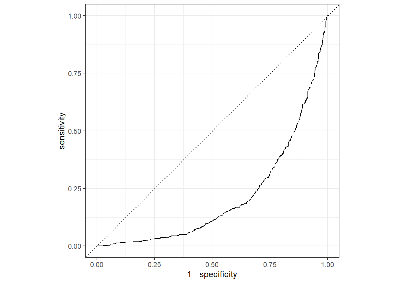
# calculate ROC_AUC score
newlj_aug %>%
  roc_auc(truth = price_above_avg, .pred_TRUE)
6 Discussion
In this article, I use the method of single-factor and multi-factor analysis and data visualization to find that the house price is related to the house location, age, floor height, number of bedrooms, building area, elevator, decoration style and house type.
Among them, elevators and hardbound drive up prices of houses of the same size. Houses of younger age tend to be more expensive. The price of houses in the middle and higher floors is higher than that in the lower floors. The price of slab building is often higher than that of tower building.
Finally, using OLS regression, I found that there was no significant relationship between building height and SQM, and found that building location could explain most of the variations in the model. The final model explains the price by 68%.
In the machine learning model, I use the median SQM of each building location to divide the sample into two groups and use the existing variables to predict whether the price of a house will above median (station and property name are not included to improve efficiency). The predicted ROC is only 0.21. Therefore, OLS model is a better choice in this report.


【推荐】国内首个AI IDE,深度理解中文开发场景,立即下载体验Trae
【推荐】编程新体验,更懂你的AI,立即体验豆包MarsCode编程助手
【推荐】抖音旗下AI助手豆包,你的智能百科全书,全免费不限次数
【推荐】轻量又高性能的 SSH 工具 IShell:AI 加持,快人一步
· AI与.NET技术实操系列:基于图像分类模型对图像进行分类
· go语言实现终端里的倒计时
· 如何编写易于单元测试的代码
· 10年+ .NET Coder 心语,封装的思维:从隐藏、稳定开始理解其本质意义
· .NET Core 中如何实现缓存的预热?
· 分享一个免费、快速、无限量使用的满血 DeepSeek R1 模型,支持深度思考和联网搜索!
· 基于 Docker 搭建 FRP 内网穿透开源项目(很简单哒)
· ollama系列01:轻松3步本地部署deepseek,普通电脑可用
· 25岁的心里话
· 按钮权限的设计及实现