
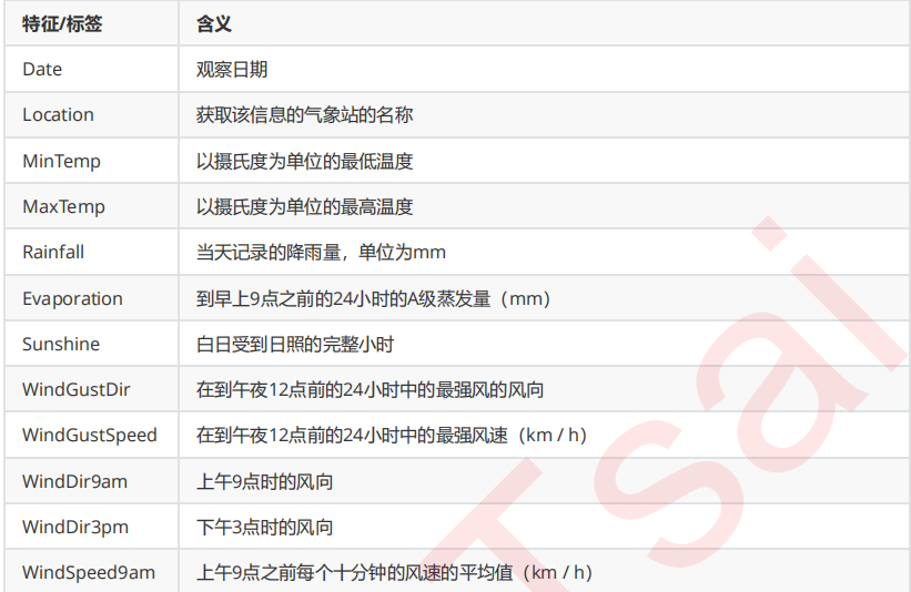
机器学习sklearn(73):算法实例(三十)分类(十七)SVM(八)sklearn.svm.SVC(七) SVC真实数据案例:预测明天是否会下雨
0 简介

Kaggle下载链接走这里:https://www.kaggle.com/jsphyg/weather-dataset-rattle-package

1 导库导数据,探索特征
导入需要的库
import pandas as pd
import numpy as np
from sklearn.model_selection import train_test_split
导入数据,探索数据
weather = pd.read_csv(r"C:\work\learnbetter\micro-class\week 8SVM (2)\data\weatherAUS5000.csv",index_col=0)
weather.head()
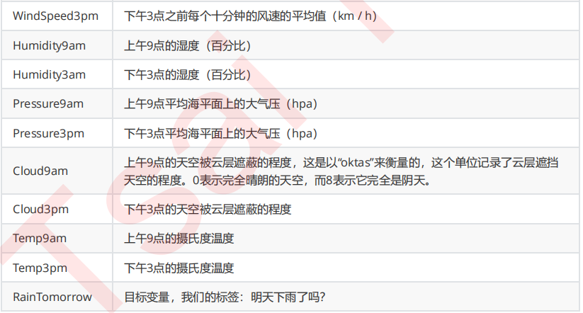
来查看一下各个特征都代表了什么:
#将特征矩阵和标签Y分开
X = weather.iloc[:,:-1] Y = weather.iloc[:,-1] X.shape
#探索数据类型
X.info()
#探索缺失值
X.isnull().mean()
#探索标签的分类
np.unique(Y)

2 分集,优先探索标签
分训练集和测试集,并做描述性统计
#分训练集和测试集
Xtrain, Xtest, Ytrain, Ytest = train_test_split(X,Y,test_size=0.3,random_state=420) #恢复索引
for i in [Xtrain, Xtest, Ytrain, Ytest]:
    i.index = range(i.shape[0])

#是否有样本不平衡问题?
Ytrain.value_counts()
Ytest.value_counts()
#将标签编码
from sklearn.preprocessing import LabelEncoder
encorder = LabelEncoder().fit(Ytrain)
Ytrain = pd.DataFrame(encorder.transform(Ytrain))
Ytest = pd.DataFrame(encorder.transform(Ytest))
3 探索特征,开始处理特征矩阵
3.1 描述性统计与异常值
#描述性统计
Xtrain.describe([0.01,0.05,0.1,0.25,0.5,0.75,0.9,0.99]).T
Xtest.describe([0.01,0.05,0.1,0.25,0.5,0.75,0.9,0.99]).T
"""
对于去kaggle上下载了数据的小伙伴们,以及坚持要使用完整版数据的(15W行)小伙伴们
如果你发现了异常值,首先你要观察,这个异常值出现的频率
如果异常值只出现了一次,多半是输入错误,直接把异常值删除
如果异常值出现了多次,去跟业务人员沟通,可能这是某种特殊表示,如果是人为造成的错误,异常值留着是没有用
的,只要数据量不是太大,都可以删除
如果异常值占到你总数据量的10%以上了,不能轻易删除。可以考虑把异常值替换成非异常但是非干扰的项,比如说用0
来进行替换,或者把异常当缺失值,用均值或者众数来进行替换
"""
#先查看原始的数据结构
Xtrain.shape
Xtest.shape
#观察异常值是大量存在,还是少数存在
Xtrain.loc[Xtrain.loc[:,"Cloud9am"] == 9,"Cloud9am"]
Xtest.loc[Xtest.loc[:,"Cloud9am"] == 9,"Cloud9am"]
Xtest.loc[Xtest.loc[:,"Cloud3pm"] == 9,"Cloud3pm"] #少数存在,于是采取删除的策略
#注意如果删除特征矩阵,则必须连对应的标签一起删除,特征矩阵的行和标签的行必须要一一对应
Xtrain = Xtrain.drop(index = 71737)
Ytrain = Ytrain.drop(index = 71737) #删除完毕之后,观察原始的数据结构,确认删除正确
Xtrain.shape
Xtest = Xtest.drop(index = [19646,29632])
Ytest = Ytest.drop(index = [19646,29632])
Xtest.shape
#进行任何行删除之后,千万记得要恢复索引
for i in [Xtrain, Xtest, Ytrain, Ytest]:
    i.index = range(i.shape[0])
Xtrain.head()
Xtest.head()
3.2 处理困难特征:日期
我们采集数据的日期是否和我们的天气有关系呢?我们可以探索一下我们的采集日期有什么样的性质:
Xtrainc = Xtrain.copy()
Xtrainc.sort_values(by="Location")
Xtrain.iloc[:,0].value_counts()
#首先,日期不是独一无二的,日期有重复
#其次,在我们分训练集和测试集之后,日期也不是连续的,而是分散的
#某一年的某一天倾向于会下雨?或者倾向于不会下雨吗?
#不是日期影响了下雨与否,反而更多的是这一天的日照时间,湿度,温度等等这些因素影响了是否会下雨
#光看日期,其实感觉它对我们的判断并无直接影响
#如果我们把它当作连续型变量处理,那算法会人为它是一系列1~3000左右的数字,不会意识到这是日期
Xtrain.iloc[:,0].value_counts().count()
#如果我们把它当作分类型变量处理,类别太多,有2141类,如果换成数值型,会被直接当成连续型变量,如果做成哑变量,我们特征的维度会爆炸

Xtrain = Xtrain.drop(["Date"],axis=1)
Xtest = Xtest.drop(["Date"],axis=1)


Xtrain["Rainfall"].head(20)
Xtrain.loc[Xtrain["Rainfall"] >= 1,"RainToday"] = "Yes"
Xtrain.loc[Xtrain["Rainfall"] < 1,"RainToday"] = "No"
Xtrain.loc[Xtrain["Rainfall"] == np.nan,"RainToday"] = np.nan
Xtest.loc[Xtest["Rainfall"] >= 1,"RainToday"] = "Yes"
Xtest.loc[Xtest["Rainfall"] < 1,"RainToday"] = "No"
Xtest.loc[Xtest["Rainfall"] == np.nan,"RainToday"] = np.nan
Xtrain.head()
Xtest.head()

int(Xtrain.loc[0,"Date"].split("-")[1]) #提取出月份
Xtrain["Date"] = Xtrain["Date"].apply(lambda x:int(x.split("-")[1]))
#替换完毕后,我们需要修改列的名称
#rename是比较少有的,可以用来修改单个列名的函数
#我们通常都直接使用 df.columns = 某个列表 这样的形式来一次修改所有的列名
#但rename允许我们只修改某个单独的列
Xtrain = Xtrain.rename(columns={"Date":"Month"})
Xtrain.head()
Xtest["Date"] = Xtest["Date"].apply(lambda x:int(x.split("-")[1]))
Xtest = Xtest.rename(columns={"Date":"Month"})
Xtest.head()

3.3 处理困难特征:地点


import time
from selenium import webdriver #导入需要的模块,其中爬虫使用的是selenium
import pandas as pd
import numpy as np
df = pd.DataFrame(index=range(len(cityname))) #创建新dataframe用于存储爬取的数据
driver = webdriver.Chrome() #调用谷歌浏览器
time0 = time.time() #计时开始
#循环开始
for num, city in enumerate(cityname): #在城市名称中进行遍历
    driver.get('https://www.google.co.uk/webhp?
hl=en&sa=X&ved=0ahUKEwimtcX24cTfAhUJE7wKHVkWB5AQPAgH')
        #首先打开谷歌主页
    time.sleep(0.3)
        #停留0.3秒让我们知道发生了什么
    search_box = driver.find_element_by_name('q') #锁定谷歌的搜索输入框
    search_box.send_keys('%s Australia Latitude and longitude' % (city)) #在输入框中输入
“城市” 澳大利亚 经纬度
    search_box.submit() #enter,确认开始搜索
    result = driver.find_element_by_xpath('//div[@class="Z0LcW"]').text #?爬取需要的经纬
度,就是这里,怎么获取的呢?
    resultsplit = result.split(" ") #将爬取的结果用split进行分割
    df.loc[num,"City"] = city #向提前创建好的df中输入爬取的数据,第一列是城市名
    df.loc[num,"Latitude"] = resultsplit[0] #第二列是纬度
    df.loc[num,"Longitude"] = resultsplit[2] #第三列是经度
    df.loc[num,"Latitudedir"] = resultsplit[1] #第四列是纬度的方向
    df.loc[num,"Longitudedir"] = resultsplit[3] #第五列是经度的方向
    print("%i webcrawler successful for city %s" % (num,city)) #每次爬虫成功之后,就打印“城 市”成功了

time.sleep(1) #全部爬取完毕后,停留1秒钟
driver.quit() #关闭浏览器
print(time.time() - time0) #打印所需的时间

cityll = pd.read_csv(r"C:\work\learnbetter\micro-class\week 8 SVM
(2)\cityll.csv",index_col=0)
city_climate = pd.read_csv(r"C:\work\learnbetter\micro-class\week 8 SVM
(2)\Cityclimate.csv")
cityll.head()
city_climate.head()

#去掉度数符号
cityll["Latitudenum"] = cityll["Latitude"].apply(lambda x:float(x[:-1]))
cityll["Longitudenum"] = cityll["Longitude"].apply(lambda x:float(x[:-1]))
#观察一下所有的经纬度方向都是一致的,全部是南纬,东经,因为澳大利亚在南半球,东半球
#所以经纬度的方向我们可以舍弃了
citylld = cityll.iloc[:,[0,5,6]]
#将city_climate中的气候添加到我们的citylld中
citylld["climate"] = city_climate.iloc[:,-1]
citylld.head()

#训练集中所有的地点
cityname = Xtrain.iloc[:,1].value_counts().index.tolist()
cityname
import time
from selenium import webdriver #导入需要的模块,其中爬虫使用的是selenium
import pandas as pd
import numpy as np
df = pd.DataFrame(index=range(len(cityname))) #创建新dataframe用于存储爬取的数据
driver = webdriver.Chrome() #调用谷歌浏览器
time0 = time.time() #计时开始
#循环开始
for num, city in enumerate(cityname): #在城市名称中进行遍历
    driver.get('https://www.google.co.uk/webhp?
hl=en&sa=X&ved=0ahUKEwimtcX24cTfAhUJE7wKHVkWB5AQPAgH')
        #首先打开谷歌主页
    time.sleep(0.3)
        #停留0.3秒让我们知道发生了什么
    search_box = driver.find_element_by_name('q') #锁定谷歌的搜索输入框
    search_box.send_keys('%s Australia Latitude and longitude' % (city)) #在输入框中输入
“城市” 澳大利亚 经纬度
    search_box.submit() #enter,确认开始搜索
    result = driver.find_element_by_xpath('//div[@class="Z0LcW"]').text #?爬取需要的经纬
度,就是这里,怎么获取的呢?
    resultsplit = result.split(" ") #将爬取的结果用split进行分割
    df.loc[num,"City"] = city #向提前创建好的df中输入爬取的数据,第一列是城市名
    df.loc[num,"Latitude"] = resultsplit[0] #第二列是经度
    df.loc[num,"Longitude"] = resultsplit[2] #第三列是纬度
    df.loc[num,"Latitudedir"] = resultsplit[1] #第四列是经度的方向
    df.loc[num,"Longitudedir"] = resultsplit[3] #第五列是纬度的方向
    print("%i webcrawler successful for city %s" % (num,city)) #每次爬虫成功之后,就打印“城 市”成功了

time.sleep(1) #全部爬取完毕后,停留1秒钟
driver.quit() #关闭浏览器
print(time.time() - time0) #打印所需的时间
df.to_csv(r"C:\work\learnbetter\micro-class\week 8 SVM (2)\samplecity.csv")
来查看一下我们爬取出的内容是什么样子:
samplecity = pd.read_csv(r"C:\work\learnbetter\micro-class\week 8 SVM
(2)\samplecity.csv",index_col=0) #我们对samplecity也执行同样的处理:去掉经纬度中度数的符号,并且舍弃我们的经纬度的方向
samplecity["Latitudenum"] = samplecity["Latitude"].apply(lambda x:float(x[:-1]))
samplecity["Longitudenum"] = samplecity["Longitude"].apply(lambda x:float(x[:-1]))
samplecityd = samplecity.iloc[:,[0,5,6]]
samplecityd.head()

#首先使用radians将角度转换成弧度
from math import radians, sin, cos, acos
citylld.loc[:,"slat"] = citylld.iloc[:,1].apply(lambda x : radians(x))
citylld.loc[:,"slon"] = citylld.iloc[:,2].apply(lambda x : radians(x))
samplecityd.loc[:,"elat"] = samplecityd.iloc[:,1].apply(lambda x : radians(x))
samplecityd.loc[:,"elon"] = samplecityd.iloc[:,2].apply(lambda x : radians(x))
import sys
for i in range(samplecityd.shape[0]):
    slat = citylld.loc[:,"slat"]
    slon = citylld.loc[:,"slon"]
    elat = samplecityd.loc[i,"elat"]
    elon = samplecityd.loc[i,"elon"]
    dist = 6371.01 * np.arccos(np.sin(slat)*np.sin(elat) +
                          np.cos(slat)*np.cos(elat)*np.cos(slon.values - elon))
    city_index = np.argsort(dist)[0]
    #每次计算后,取距离最近的城市,然后将最近的城市和城市对应的气候都匹配到samplecityd中
    samplecityd.loc[i,"closest_city"] = citylld.loc[city_index,"City"]
    samplecityd.loc[i,"climate"] = citylld.loc[city_index,"climate"] #查看最后的结果,需要检查城市匹配是否基本正确
samplecityd.head()
#查看气候的分布
samplecityd["climate"].value_counts()
#确认无误后,取出样本城市所对应的气候,并保存
locafinal = samplecityd.iloc[:,[0,-1]]
locafinal.head()
locafinal.columns = ["Location","Climate"] #在这里设定locafinal的索引为地点,是为了之后进行map的匹配
locafinal = locafinal.set_index(keys="Location")
locafinal.to_csv(r"C:\work\learnbetter\micro-class\week 8 SVM (2)\samplelocation.csv")
locafinal.head()

#是否还记得训练集长什么样呢?
Xtrain.head()
#将location中的内容替换,并且确保匹配进入的气候字符串中不含有逗号,气候两边不含有空格
#我们使用re这个模块来消除逗号
#re.sub(希望替换的值,希望被替换成的值,要操作的字符串)
#x.strip()是去掉空格的函数
import re
Xtrain["Location"] = Xtrain["Location"].map(locafinal.iloc[:,0]).apply(lambda
x:re.sub(",","",x.strip()))
Xtest["Location"] = Xtest["Location"].map(locafinal.iloc[:,0]).apply(lambda
x:re.sub(",","",x.strip()))
#修改特征内容之后,我们使用新列名“Climate”来替换之前的列名“Location”
#注意这个命令一旦执行之后,就再没有列"Location"了,使用索引时要特别注意
Xtrain = Xtrain.rename(columns={"Location":"Climate"})
Xtest = Xtest.rename(columns={"Location":"Climate"})
Xtrain.head()
Xtest.head()

3.4 处理分类型变量:缺失值

#查看缺失值的缺失情况
Xtrain.isnull().mean()
#首先找出,分类型特征都有哪些
cate = Xtrain.columns[Xtrain.dtypes == "object"].tolist()
#除了特征类型为"object"的特征们,还有虽然用数字表示,但是本质为分类型特征的云层遮蔽程度
cloud = ["Cloud9am","Cloud3pm"]
cate = cate + cloud
cate
#对于分类型特征,我们使用众数来进行填补
from sklearn.impute import SimpleImputer
si = SimpleImputer(missing_values=np.nan,strategy="most_frequent") #注意,我们使用训练集数据来训练我们的填补器,本质是在生成训练集中的众数
si.fit(Xtrain.loc[:,cate])
#然后我们用训练集中的众数来同时填补训练集和测试集
Xtrain.loc[:,cate] = si.transform(Xtrain.loc[:,cate])
Xtest.loc[:,cate] = si.transform(Xtest.loc[:,cate])
Xtrain.head()
Xtest.head()
#查看分类型特征是否依然存在缺失值
Xtrain.loc[:,cate].isnull().mean()
Xtest.loc[:,cate].isnull().mean()
3.5 处理分类型变量:将分类型变量编码


#将所有的分类型变量编码为数字,一个类别是一个数字
from sklearn.preprocessing import OrdinalEncoder
oe = OrdinalEncoder()
#利用训练集进行fit
oe = oe.fit(Xtrain.loc[:,cate])
#用训练集的编码结果来编码训练和测试特征矩阵
#在这里如果测试特征矩阵报错,就说明测试集中出现了训练集中从未见过的类别
Xtrain.loc[:,cate] = oe.transform(Xtrain.loc[:,cate])
Xtest.loc[:,cate] = oe.transform(Xtest.loc[:,cate])
Xtrain.loc[:,cate].head()
Xtest.loc[:,cate].head()
3.6 处理连续型变量:填补缺失值

col = Xtrain.columns.tolist()
for i in cate:
    col.remove(i)
col
#实例化模型,填补策略为"mean"表示均值
impmean = SimpleImputer(missing_values=np.nan,strategy = "mean") #用训练集来fit模型
impmean = impmean.fit(Xtrain.loc[:,col])
#分别在训练集和测试集上进行均值填补
Xtrain.loc[:,col] = impmean.transform(Xtrain.loc[:,col])
Xtest.loc[:,col] = impmean.transform(Xtest.loc[:,col])
Xtrain.head()
Xtest.head()
3.7 处理连续型变量:无量纲化

col.remove("Month")
col
from sklearn.preprocessing import StandardScaler
ss = StandardScaler()
ss = ss.fit(Xtrain.loc[:,col])
Xtrain.loc[:,col] = ss.transform(Xtrain.loc[:,col])
Xtest.loc[:,col] = ss.transform(Xtest.loc[:,col])
Xtrain.head()
Xtest.head()
Ytrain.head()
Ytest.head()

4 建模与模型评估
from time import time
import datetime
from sklearn.svm import SVC
from sklearn.model_selection import cross_val_score
from sklearn.metrics import roc_auc_score, recall_score
Ytrain = Ytrain.iloc[:,0].ravel()
Ytest = Ytest.iloc[:,0].ravel()
#建模选择自然是我们的支持向量机SVC,首先用核函数的学习曲线来选择核函数
#我们希望同时观察,精确性,recall以及AUC分数
times = time() #因为SVM是计算量很大的模型,所以我们需要时刻监控我们的模型运行时间
for kernel in ["linear","poly","rbf","sigmoid"]:
    clf = SVC(kernel = kernel
             ,gamma="auto"
             ,degree = 1
             ,cache_size = 5000
             ).fit(Xtrain, Ytrain)
    result = clf.predict(Xtest)
    score = clf.score(Xtest,Ytest)
    recall = recall_score(Ytest, result)
    auc = roc_auc_score(Ytest,clf.decision_function(Xtest))
    print("%s 's testing accuracy %f, recall is %f', auc is %f" % (kernel,score,recall,auc))
    print(datetime.datetime.fromtimestamp(time()-times).strftime("%M:%S:%f"))

5 模型调参
5.1 最求最高Recall

times = time()
for kernel in ["linear","poly","rbf","sigmoid"]:
    clf = SVC(kernel = kernel
             ,gamma="auto"
             ,degree = 1
             ,cache_size = 5000
             ,class_weight = "balanced"
             ).fit(Xtrain, Ytrain)
    result = clf.predict(Xtest)
    score = clf.score(Xtest,Ytest)
    recall = recall_score(Ytest, result)
    auc = roc_auc_score(Ytest,clf.decision_function(Xtest))
    print("%s 's testing accuracy %f, recall is %f', auc is %f" % (kernel,score,recall,auc))
    print(datetime.datetime.fromtimestamp(time()-times).strftime("%M:%S:%f"))

times = time()
clf = SVC(kernel = "linear"
         ,gamma="auto"
         ,cache_size = 5000
         ,class_weight = {1:10} #注意,这里写的其实是,类别1:10,隐藏了类别0:1这个比例
         ).fit(Xtrain, Ytrain)
result = clf.predict(Xtest)
score = clf.score(Xtest,Ytest)
recall = recall_score(Ytest, result)
auc = roc_auc_score(Ytest,clf.decision_function(Xtest))
print("testing accuracy %f, recall is %f', auc is %f" %(score,recall,auc))
print(datetime.datetime.fromtimestamp(time()-times).strftime("%M:%S:%f"))

5.2 追求最高准确率

valuec = pd.Series(Ytest).value_counts()
valuec
valuec[0]/valuec.sum()

#查看模型的特异度
from sklearn.metrics import confusion_matrix as CM
clf = SVC(kernel = "linear"
         ,gamma="auto"
         ,cache_size = 5000
         ).fit(Xtrain, Ytrain)
result = clf.predict(Xtest)
cm = CM(Ytest,result,labels=(1,0))
cm
specificity = cm[1,1]/cm[1,:].sum()
specificity #几乎所有的0都被判断正确了,还有不少1也被判断正确了

irange = np.linspace(0.01,0.05,10)
for i in irange:
    times = time()
    clf = SVC(kernel = "linear"
             ,gamma="auto"
             ,cache_size = 5000
             ,class_weight = {1:1+i}
             ).fit(Xtrain, Ytrain)
    result = clf.predict(Xtest)
    score = clf.score(Xtest,Ytest)
    recall = recall_score(Ytest, result)
    auc = roc_auc_score(Ytest,clf.decision_function(Xtest))
    print("under ratio 1:%f testing accuracy %f, recall is %f', auc is %f" % (1+i,score,recall,auc))
    print(datetime.datetime.fromtimestamp(time()-times).strftime("%M:%S:%f"))

irange_ = np.linspace(0.018889,0.027778,10)
for i in irange_:
    times = time()
    clf = SVC(kernel = "linear"
             ,gamma="auto"
             ,cache_size = 5000
             ,class_weight = {1:1+i}
             ).fit(Xtrain, Ytrain)
    result = clf.predict(Xtest)
    score = clf.score(Xtest,Ytest)
    recall = recall_score(Ytest, result)
    auc = roc_auc_score(Ytest,clf.decision_function(Xtest))
    print("under ratio 1:%f testing accuracy %f, recall is %f', auc is %f" % (1+i,score,recall,auc))
    print(datetime.datetime.fromtimestamp(time()-times).strftime("%M:%S:%f"))

from sklearn.linear_model import LogisticRegression as LR
logclf = LR(solver="liblinear").fit(Xtrain, Ytrain)
logclf.score(Xtest,Ytest)
C_range = np.linspace(3,5,10)
for C in C_range:
    logclf = LR(solver="liblinear",C=C).fit(Xtrain, Ytrain)
    print(C,logclf.score(Xtest,Ytest))

5.3 追求平衡

###======【TIME WARNING:10mins】======###
import matplotlib.pyplot as plt
C_range = np.linspace(0.01,20,20)
recallall = []
aucall = []
scoreall = []
for C in C_range:
    times = time()
    clf = SVC(kernel = "linear",C=C,cache_size = 5000
             ,class_weight = "balanced"
             ).fit(Xtrain, Ytrain)
    result = clf.predict(Xtest)
    score = clf.score(Xtest,Ytest)
    recall = recall_score(Ytest, result)
    auc = roc_auc_score(Ytest,clf.decision_function(Xtest))
    recallall.append(recall)
    aucall.append(auc)
    scoreall.append(score)
    print("under C %f, testing accuracy is %f,recall is %f', auc is %f" % (C,score,recall,auc))
    print(datetime.datetime.fromtimestamp(time()-times).strftime("%M:%S:%f"))

print(max(aucall),C_range[aucall.index(max(aucall))])
plt.figure()
plt.plot(C_range,recallall,c="red",label="recall")
plt.plot(C_range,aucall,c="black",label="auc")
plt.plot(C_range,scoreall,c="orange",label="accuracy")
plt.legend()
plt.show()

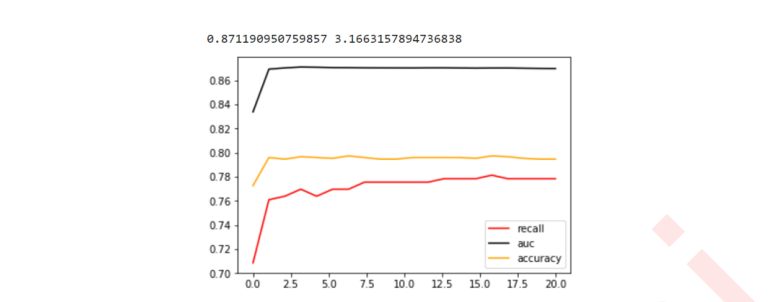

times = time()
clf = SVC(kernel = "linear",C=3.1663157894736838,cache_size = 5000
         ,class_weight = "balanced"
         ).fit(Xtrain, Ytrain)
result = clf.predict(Xtest)
score = clf.score(Xtest,Ytest)
recall = recall_score(Ytest, result)
auc = roc_auc_score(Ytest,clf.decision_function(Xtest))
print("testing accuracy %f,recall is %f', auc is %f" % (score,recall,auc))
print(datetime.datetime.fromtimestamp(time()-times).strftime("%M:%S:%f"))

from sklearn.metrics import roc_curve as ROC
import matplotlib.pyplot as plt
FPR, Recall, thresholds = ROC(Ytest,clf.decision_function(Xtest),pos_label=1)
area = roc_auc_score(Ytest,clf.decision_function(Xtest))
plt.figure()
plt.plot(FPR, Recall, color='red',
         label='ROC curve (area = %0.2f)' % area)
plt.plot([0, 1], [0, 1], color='black', linestyle='--')
plt.xlim([-0.05, 1.05])
plt.ylim([-0.05, 1.05])
plt.xlabel('False Positive Rate')
plt.ylabel('Recall')
plt.title('Receiver operating characteristic example')
plt.legend(loc="lower right")
plt.show()
以此模型作为基础,我们来求解最佳阈值:
maxindex = (Recall - FPR).tolist().index(max(Recall - FPR))
thresholds[maxindex]
基于我们选出的最佳阈值,我们来认为确定y_predict,并确定在这个阈值下的recall和准确度的值:
from sklearn.metrics import accuracy_score as AC
times = time()
clf = SVC(kernel = "linear",C=3.1663157894736838,cache_size = 5000
         ,class_weight = "balanced"
         ).fit(Xtrain, Ytrain)
prob = pd.DataFrame(clf.decision_function(Xtest))
prob.loc[prob.iloc[:,0] >= thresholds[maxindex],"y_pred"]=1
prob.loc[prob.iloc[:,0] < thresholds[maxindex],"y_pred"]=0
prob.loc[:,"y_pred"].isnull().sum()
#检查模型本身的准确度
score = AC(Ytest,prob.loc[:,"y_pred"].values)
recall = recall_score(Ytest, prob.loc[:,"y_pred"])
print("testing accuracy %f,recall is %f" % (score,recall))
print(datetime.datetime.fromtimestamp(time()-times).strftime("%M:%S:%f"))

6 SVM总结&结语

本文来自博客园,作者:秋华,转载请注明原文链接:https://www.cnblogs.com/qiu-hua/p/14960826.html
