windows11安装Graphviz

一  下载地址

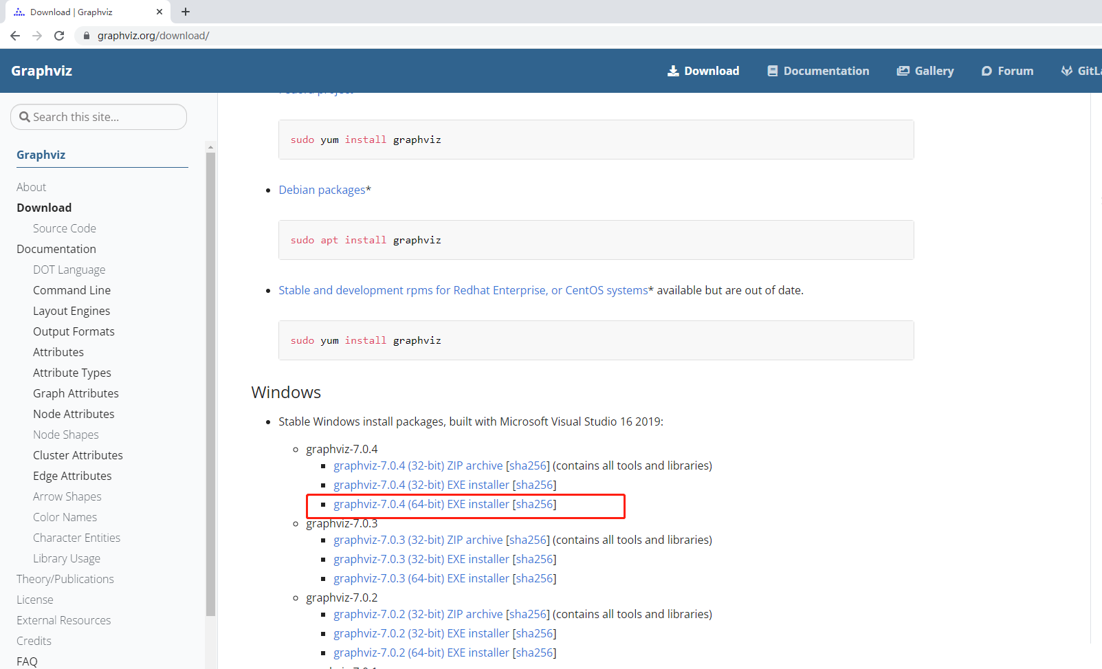
https://graphviz.org/download/

我选择的是64位的7.0.4版本。

 

 

 

 

 

二、安装步骤

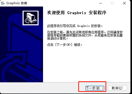
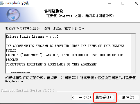
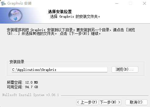
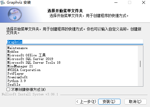
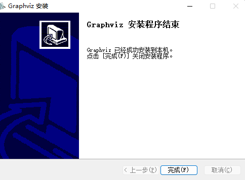
2.1 正常安装

就是一直按下一步就行。

 

 

 

 

 

 

 

 

 

 

 

 

 

 

 

 

 

 

 

 

 

 

 

 

 

 

 

 

 

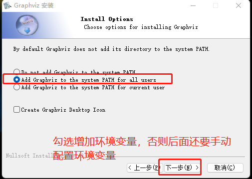
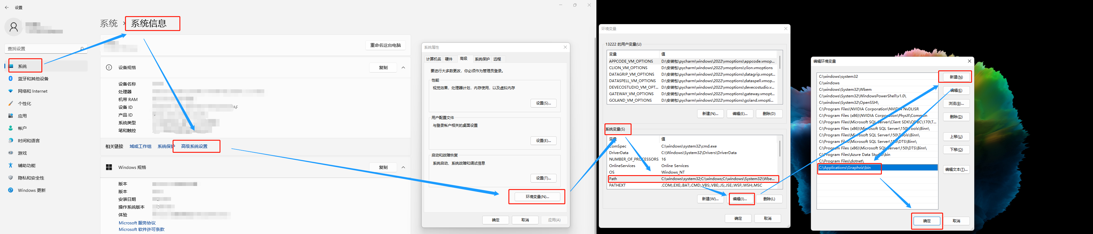
2.2 配置环境变量

如果没有配置环境变量，可按照下图配置环境变量

注意路径，找到安装路径的bin所有绝对路径，复制过去就行了

 

 

 

 

 

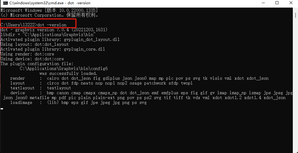
2.3 检查是否配置成功

win+R 调出运行对话框，

输入dot -version 查看是否安装成功

 

 

 

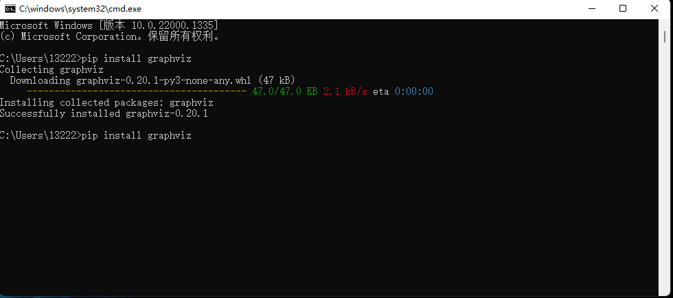
2.4  安装graphviz包

 

 

 

 

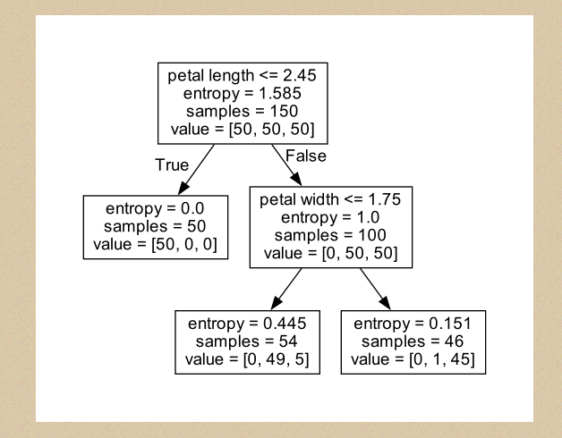
三、展示

import graphviz
import numpy as np
import pandas as pd
import matplotlib.pyplot as plt
from sklearn.model_selection import train_test_split
from sklearn.model_selection import GridSearchCV
from matplotlib.colors import ListedColormap
from sklearn import datasets
from scipy.stats import pearsonr
from sklearn.tree import DecisionTreeClassifier, export_graphviz

# 获取数据集
iris = datasets.load_iris()
# (150, 4) (150,)
# print(iris['data'].shape, iris['target'].shape)
df = pd.DataFrame(data=iris.data, columns=iris.feature_names)
# print(iris)
print(df)
# 使用皮尔逊系数确认哪些列与标签强相关
dict_pear = {}
for column in df.columns:
    dict_pear[column] = np.round(pearsonr(df[column], iris['target'])[0], 4)
print(dict_pear)
# {'sepal length (cm)': 0.7826, 'sepal width (cm)': -0.4267, 'petal length (cm)': 0.949, 'petal width (cm)': 0.9565}
# 可以发现，petal length (cm)': 0.949, 'petal width (cm)': 0.9565 相关度较高,也为了可视化方便，选取后面两个
X = np.array(df.iloc[:, 2:])
# y是目标值 0,1,2
y = iris['target']


X_train, X_test, y_train, y_test = train_test_split(X, y, test_size=0.25, random_state=2 )
dt_clf = DecisionTreeClassifier()
# 决策树,max_depth 最高的深度,先设置2后面在调整,criterion:默认基尼系数, 建议采用交叉熵
gc = GridSearchCV(estimator=dt_clf, param_grid={'max_depth':[1, 2, 3, 4], 'criterion':['entropy'], 'random_state':[2]},cv=2)

gc.fit(X_train, y_train)

# 交叉验证与网格搜索相关结果如下：
print("最优模型参数", gc.best_estimator_)
# DecisionTreeClassifier(criterion='entropy', max_depth=2, random_state=2)


# 可视化
plt.scatter(X[y == 0, 0], X[y == 0, 1])
# 采用目标值来筛选样本,吧样本的第0个和第1个特征值分别设置为散点图的x与y轴
plt.scatter(X[y == 1, 0], X[y == 1, 1])
plt.scatter(X[y == 2, 0], X[y == 2, 1])
plt.show()


# 采用等高线刻画出分类图,此部分与二叉树原理无关,感兴趣同事可以参考：np.meshgrid  np.c_ plt.contourf API
def plot_decistion_boundary(model, axis):
    x0, x1 = np.meshgrid(
        np.linspace(axis[0], axis[1], int((axis[1] - axis[0])) * 100).reshape(-1, 1),
        np.linspace(axis[2], axis[3], int((axis[3] - axis[2])) * 100).reshape(-1, 1)
    )
    X_new = np.c_[x0.ravel(), x1.ravel()]
    y_predict = model.predict(X_new)
    zz = y_predict.reshape(x0.shape)
    custom_cmap = ListedColormap(['#EF9A9A', '#FFF59D', '#90CAF9'])
    plt.contourf(x0, x1, zz, cmap=custom_cmap)

# 将最优解带入到决策树中，不再设训练集与测试集
clf = DecisionTreeClassifier(criterion='entropy',random_state=2, max_depth=2)
clf.fit(X, y)
export_graphviz(decision_tree=clf,out_file="../data/iris.dot", feature_names=['petal length', 'petal width'])
# 设置等高线的边界
plot_decistion_boundary(clf, axis=[0.5, 7.5, 0, 3])
plt.scatter(X[y == 0, 0], X[y == 0, 1])
plt.scatter(X[y == 1, 0], X[y == 1, 1])
plt.scatter(X[y == 2, 0], X[y == 2,1])
plt.show()


with open("../data/iris.dot") as f:
    dot_graph = f.read()
dot = graphviz.Source(dot_graph)
dot.view()