

摘要
Knowledge Graph Completion (KGC)旨在补全Knowledge Graphs (KGs)的缺失部分,尤其是multimodal KGs (MKGs,多模态知识图谱),主要是因为多模态语料库的积累不足导致的关系不完整。负采样面临着一个独特的挑战,即如何在学习多模态之间的互补语义作为额外上下文的过程中对KG关系的影响进行建模。
本文提出了一种用于多模态KGC任务的多模态关系增强负采样(MMRNS)框架。一种新的知识引导的跨模态注意(KCA)机制,该机制通过整合关系嵌入为视觉和文本特征提供双向注意。然后,在将KCA机制与对比学习相结合的基础上,设计了一种有效的对比语义采样器。通过这种方式,可以学习到正负样本之间语义特征的更相似表示,以及不同关系下正负样本之间更多样化的表示。然后,利用masked gumbel-softmax优化机制来解决采样过程的不可微性,与传统的采样策略相比,该机制提供了有效的参数优化。
1.引言
针对多模态场景的知识图补全(KGC)解决方案引起了广泛关注,该解决方案旨在自动推断缺失的事实。具体来说,之前的KGC方法主要试图通过均匀采样来构建负样本,这在训练的后期会遇到梯度消失的问题。因此,迫切需要一种针对多模态KG的专门设计的负采样策略。目前的技术主要侧重于结构知识,而丰富的多模态线索没有得到充分利用,这严重降低了有效性。
此外,在共同学习多模态属性时,KG中的关系可能起着重要作用,因为它们可以作为额外的上下文指导多模态之间互补语义的学习。
为了解决这个问题,我们提出了一种新的知识引导的跨模态注意(KCA)机制,该机制整合了同一实体的多种关系,以估计多模态语义特征的双向注意权重。
具体而言,设计了两个部分,其中一部分通过相互关注关系无关特征来总结多模态线索,另一部分通过嵌入关系引导特征的关系来双向联合推理多模态注意力。在KGs中普遍存在1-to-Many关系,例如获奖的关系可能将格莱美奖和许多著名歌手作为该奖项的获得者联系起来,自然会在KGs中产生一些正向的三元组,即两个相似的实体可能都是正的。这一现象促使我们捕捉正样本之间语义特征的相似性,以及1-to-Many关系下负样本之间的多样性。因此,基于KCA机制,引入对比损失来构建对比语义采样器,旨在进一步学习正负样本之间的多模态语义相似/差异表示,以估计采样分布。
沿着这一思路,在本文中,我们设计了一个多模态关系增强负采样(MMRNS)框架,通过联合利用多模态数据和复杂的KG关系来增强实体的语义表示,并通过对比语义采样器增强KCA机制,从而找出困难负样本。之后,考虑到不可微的采样过程可能导致难以通过优化KGC模型来端到端地细化采样网络参数,进一步调整了掩码gumbel-softmax工具,以实现采样网络的可微解。具体来说,在gumbel-softmax的基础上集成了掩码操作,以确保在正向传播过程中可以滤除正样本,在反向传播过程中返回梯度。此外,利用随迭代次数变化的可变因素来动态解决早期和后期训练阶段的勘探开发权衡问题。本文贡献总结如下:
- 提出了一种新的知识引导注意力机制,通过对比语义采样器进行增强,在复杂KG关系的指导下进行跨模态语义学习。
- 采用掩码gumbel-softmax工具实现梯度反向传播,通过KGC模型损失优化网络参数。
- 通过总结多模态线索和揭示复杂关系,广泛的评估证明了我们的负采样方法的有效性和稳健性。
2.相关工作
2.1 知识图补全(KGC)
知识图补全(KGC)旨在预测知识图中缺失的部分。一组是提出将关系建模为学习实体和关系嵌入的头尾实体之间的距离。另一组技术是语义匹配模型。然而,大多数现有技术都专注于为KGC设计更好的评分函数,但忽略了负采样策略的重要性,这可能会限制这些方法性能的进一步提高。
2.2 KGC的负采样
找到困难样本的核心点要么是使用KGs的结构知识,要么是试图使用负样本分数。然而,它们仍然存在两个问题:
- 由于KG的不完整性,用结构知识训练的模型只能提供有限的负分数信息;
- 需要一种更有效的参数优化策略来利用KGC模型的负分数。
2.3 多模态知识图谱
目前仍然缺乏专门针对MKG设计的负采样策略。在本文中,为了识别困难负样本,我们提出了一种新的知识引导的跨模态注意,并构建了一个对比语义采样器,以关系为指导来增强多模态实体的语义表示。同时,采用了一种新的优化策略来有效地更新多模态采样网络的参数。
3.方法论
3.1 准备工作和问题定义
给定知识图谱$\mathscr{G} = {(h,r,t)} \subseteq \mathcal{E}\times\mathcal{R}\times\mathcal{E} $, \(\mathcal{E}\) 表示实体集,\(\mathcal{R}\) 表示关系集。此外,我们用$ t \in \mathbb{R}^{d_{emd}}$ 和 $ r \in \mathbb{R}^{d_{emd}}$表示实体嵌入和关系嵌入。 用 $ e_i= \mathbb{R}^{d_i \times d_N}$ 表示图像特征, \(e_t = \mathbb{R}^{d_t \times d_M}\) 表示文本特征,两者用来描述多模态线索。
通过这种方法,KGC任务可以被建模为一个排名问题,给定一个正向的三元组 \((h,r,t^+)\) 和几个负样本\((h,r,t^-)\)KGC模型旨在通过有效的评分函数提高正三元组的得分,并降低负三元组的分数。沿着这一思路,我们的采样策略的目标是利用正三元组和相应的多模态数据来最大化困难负样本\(t^-\)的采样概率,这些样本在语义上与正样本相似,以提高模型的判别能力。
3.2基于知识引导的跨模态注意力机制(KCA,Knowledge-guided Cross-modal Attention)
该机制通过整合多种关系来学习跨模态双向注意权重。
具体来说,KCA首先试图捕捉不同模态(即图像和文本)之间的相互作用,旨在同时突出跨模态数据之间的相同语义特征,以学习关系无关的特征。使用跨模态特征来表示关系无关特征,这些特征在不同的关系下都很重要,可以识别困难样本。
同时,KCA在描述了多模态交互后进一步整合关系信息,以指导模型提取出多模态语义特征来学习关系-引导特征。如,当关系为“获奖”时,KCA旨在增强歌手和音乐等属性的跨模态注意力。值得注意的是,关系作为一种明确数据,包含有限和粗粒度的标签信息,通常与图像和文本没有语义相似性或相关性。因此,在引入关系进行引导时,我们首先对文本和视觉特征的交互进行建模,然后引入关系嵌入来分别引导图像和文本的跨模态注意力权重。(关系和实体是没有相关性的,所以要在对多模态特征建模之后,才能进行嵌入)。

考虑到视觉特征 \(e_i\) 和文本特征 \(e_t\),它们首先被输入一个完整的连接网络,用于非线性映射和维度统一:
$\hat{e}_i$和$\hat{e}_t$前向传播对应源码
        # 进行维度统一
        if self.args.pre_sample_num:
            text_emb = self.relu(self.linear_text(self.ent_text_emb[pre_sample]))  # e x 4 x 200
            img_emb = self.relu(self.linear_img(self.ent_img_emb[pre_sample]))  # e x 24 x 200
        else:
            text_emb = self.relu(self.linear_text(self.ent_text_emb))  # e x 4 x 200
            img_emb = self.relu(self.linear_img(self.ent_img_emb))  # e x 24 x 200
跨模态特征,前向传播对应源码
        # 得出跨模态特征
        cross_mat = torch.matmul(img_emb,text_emb.permute(0,2,1))  # e x 24 x 4
1. 文本引导的视觉注意力
2. 关系-文本引导的视觉注意力
3. 关系-图像引导的文本注意力
4. 图像引导的文本注意力
如下图所示:

MMRNS的框架图:

在①中,KCA对\(M\)进行归一化,以得到受每个文本影响的视觉注意力权重。随后注意力权重与图像特征\(\hat{e}_i\)相乘得到与关系无关(relation-irrelevant)的视觉表示\(e^i_{ir}\),这对于许多关系类型都是通用的:
$e^i_{ir}$对应源码
# 得出与关系无关的视觉表示
        img_att = torch.matmul(torch.softmax(cross_mat.permute(0,2,1),dim=2),img_emb)  # e x 4 x 200
$e_{gu}^i$对应代码
# 计算得出引导关系
        rel_guided_img = torch.sigmoid(self.linear_rel1(relation_emb)).view(batchsize,24,4) # B x 24 x 4
        # 图中的 跨模态特征有转置 但实际没有
        rel_guided_img = torch.mul(rel_guided_img.unsqueeze(1).expand(-1,num_entity,-1,-1),cross_mat)  # B x e x 24 x 4
        # 得出关系引导视觉表示
        img_att_rel_guided = torch.matmul(rel_guided_img.permute(0,1,3,2),img_emb) # B x e x 4 x 200
$e^r_i$和$e_t^r$对应源码
# 计算得出引导关系
        rel_guided_img = torch.sigmoid(self.linear_rel1(relation_emb)).view(batchsize,24,4) # B x 24 x 4
# 计算引导关系
        rel_guided_text = torch.sigmoid(self.linear_rel2(relation_emb)).view(batchsize,24,4)
$e^i_{kca}$对应源码
# 最终得出知识引导的视觉表示
        img_att_all = self.layernorm(img_att_rel_guided) + self.layernorm(img_att)  # # B x e x 4 x 200
层规范化,\(H\)表示隐藏单元数量,在层规范化下,层中所有的隐藏单元共享相同的规范化项\(\mu\)和\(\sigma\):
同样可以得到知识引导的文本表示\(e^t_{kca}\)。
$e^t_{kca}$对应源码
        text_att = torch.matmul(torch.softmax(cross_mat,dim=2),text_emb)  # e x 24 x 200
        # 计算引导关系
        rel_guided_text = torch.sigmoid(self.linear_rel2(relation_emb)).view(batchsize,24,4)
        rel_guided_text = torch.mul(rel_guided_text.unsqueeze(1).expand(-1,num_entity,-1,-1),cross_mat)  # B x e x 24 x 4
        text_att_rel_guided = torch.matmul(rel_guided_text,text_emb)  # B x e x 24 x 200
        text_att_all = self.layernorm(text_att_rel_guided) + self.layernorm(text_att) # # B x e x 24 x 200
3.3对比语义采样器(Contrastive Semantic Sampler)
然后,进一步构建了一个对比语义采样器来计算负样本的采样分布。采样器首先应用预训练模型提取语义特征,然后使用KCA机制在关系的引导下对多模态交互进行建模。采样器的核心点是通过挖掘正样本和负样本之间的异同来进一步学习多模态语义表示。

3.3.1 特征提取
首先通过BEiT提取初步的视觉特征,该特征可用于学习语义区域和对象边界。将平均池应用于语义视觉表示,以降低计算复杂度。过SBERT提取了初步的文本特征。此外,应用切割和填充来使表示张量具有相同的维度。于实体也是结构嵌入的关系,我们只需将它们连接起来并馈送到一个完整的连接网络中,以整合关系信息。
$e_s$对应源码
        # 整合关系
        relation_emb = relation_emb.unsqueeze(1).expand(-1,num_entity,-1)
        t = t.unsqueeze(0).expand(batchsize,-1,-1)
        att = torch.cat([t,relation_emb],dim=2)
        # 论文图中没有画出RELU的操作
        att = self.relu(self.linear1(att))
        att = torch.sigmoid(self.linear3(att)) #  B x Entity x dim
        t_att = t * att  #  B x Entity x dim
3.3.2 余弦相似性(Cosine Similarity)
正样本和负样本的图像文本对的初步特征都分别输入到KCA中。正负样本的KCA共享参数,两个实体视觉表示之间的视觉特征相似性\(z_i\)和\(z_j\)用余弦相似度进行衡量。\(\delta\)防止分母为0.
计算余弦相似度对应代码
      # 计算余弦相似度
        simil_img = torch.matmul(img_att_all,pos_img_emb.unsqueeze(-1)).squeeze(-1) # batchsize x nEntity
        simil_img = torch.div(simil_img,(torch.norm(img_att_all,2,dim=2)*torch.norm(pos_img_emb,2,dim=1).unsqueeze(1) ).detach() + 1e-10  )
        simil_text = torch.matmul(text_att_all,pos_text_emb.unsqueeze(-1)).squeeze(-1)
        simil_text = torch.div(simil_text,(torch.norm(text_att_all,2,dim=2)*torch.norm(pos_text_emb,2,dim=1).unsqueeze(1) ).detach() + 1e-10 )
        simil_t = torch.matmul(t_att,pos_tail_emb.unsqueeze(-1)).squeeze(-1)
        simil_t = torch.div(simil_t,(torch.norm(t_att,2,dim=2)*torch.norm(pos_tail_emb,2,dim=1).unsqueeze(1)).detach() + 1e-10 )
3.3.3 对比损失(Contrastive Loss)
损失函数使用相似性作为输入,输入多个正样本。这个损失函数的目的是最小化正样本之间的差距,扩大负样本和正样本的差距。框架中集成了自对抗技术,以进一步提高模型性能。对于第\(i\)个三元组的损失权重\(p(h_i,r,t_i)\)由KGC模型计算得出。未采样的三元组权重设置为\(\frac{1}{|\epsilon|}\)
其中\(S\)是采样三元组的集合,\(\alpha\)是采样温度。特征相似性的最终对比损失函数如下:
此处\(P\)代表正样本,\(N\)是负样本。文本和结构特征的相似度通过等式(8)计算,\(l_{con}^t\)和\(l_{con}^s\)通过等式(10)计算。最终的损失函数就是去平均值:
3.4 Masked Gumbel-Softmax
解释如何使用所提出的可微分采样方法,该方法将掩模操作与gumbel-softmax,以确保有效的梯度反向传播。掩模操作旨在克服将gumbel softmax引入KGC采样过程的问题。
3.4.1 Gumbel-Softmax
由于分类分布的采样过程独立于优化过程,KGC模型的梯度无法反向传播到采样网络。因此,对比语义采样器的可训练参数无法在KGC模型训练阶段以端到端的方式进行优化。为了实现梯度反向传播,我们引入了gumbel-softmax重新参数化技巧,该技巧通过使用softmax函数作为argmax的可微近似:\(y = softmax(\frac{(log(p)+g)}{\tau})\),产生了一个连续分布,可以从离散概率分布中近似样本.此处,每一个元素\(g_i\)在自于\(g\)是从标准Gumbel分布中取得。
3.4.2 Masked vector
考虑到图像、文本和结构中正负样本的语义相似性分别用于计算概率分布,我们利用softmax将相似性转化为采样概率:
此处的\(SF(\cdot)\)代表softmax函数,\(\epsilon\)是一个平衡参数(之后再解释)。然而,\(p\)不是最终的采样分布,一对多的关系再KGs中非常常见,并非所有的实体都可以视为负样本。所以说,最常用的方法是过滤掉正样本,这一目标的常见方法就是将概率分布中正样本的分布设置为0,但这将使gumbel-softmax不可微,这与我们的目的相矛盾。因此,文中提出了一个不可微的掩码向量,其中负位置的值被设置为1.0,正位置的值设置为非常接近零的数字。概率分布\(p\)逐个元素乘以掩码向量。由于\(log\)函数可以降低计算复杂度,因此乘法可以用加法代替。以下是masked gumbel-softmax:
\(y_m\)即使取样结果,值得注意的是,掩码向量也有利于实现无需替换的采样。总损失\(L\)由KGC模型的损失\(L_{kgc}\)和取样损失\(L_{con}\),损失率\(\beta\)在4.5解析。
3.4.3 Exploration and Exploitation
在这里,考虑到采样策略在不同训练阶段的适应性,我们进一步定义了一个exploration and exploitation factor \(\epsilon\),动机是为了在早期的训练阶段中学习困难和简单的样本。并在后期训练阶段更加注重困难样本的利用。\(\epsilon\)的值随着迭代次数的增加而减小。\(\epsilon_0\)的详细作用在4.5中详细讨论。
4.实验
4.5超参数分析
4.5.2 Parameters of MMRNS

对于exploration-exploitation factor \(\beta\)和损失率\(\epsilon\)。\(\epsilon\)表示采样网络给出的采样分布的利用程度。当\(\epsilon_0\)等于1时表现最好,当等于3时性能显著下降,这表明文中的采样方法有助于实现更好的性能。更重要的是,\(\epsilon\)值越高,曲线越平滑。\(\epsilon\)值非常大的采样分布将近似均匀分布。损失率\(\beta\)负责将损失\(L_{kgc}\)和损失\(L_{con}\)的影响调整为采样网路的可训练参数,我们观察到,当损失率等于0.005时,性能最佳。
代码解析
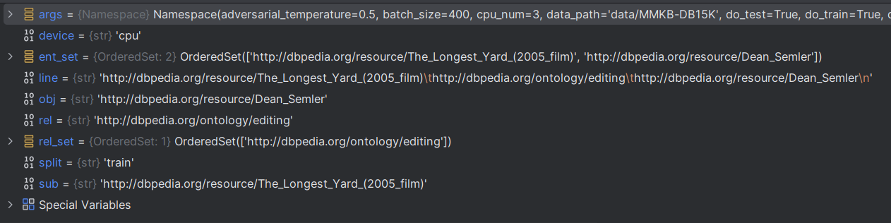
数据处理
# 集合并且会储存元素的顺序
ent_set, rel_set = OrderedSet(), OrderedSet()
# 按顺序打开文本文件
for split in ['train', 'test', 'valid']:
for line in open('{}/{}.txt'.format(args.data_path, split), encoding='utf-8'):
# 对每一行文本strip()去除尾部换行符,并根据split('\t')进行切割
sub, rel, obj = line.strip().split('\t')
# 集合元素添加
ent_set.add(sub)
rel_set.add(rel)
ent_set.add(obj)
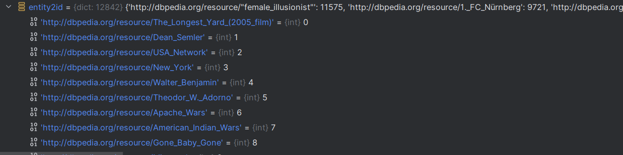
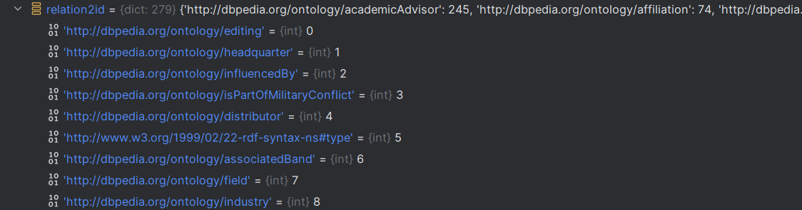
# 根据ent_set去构建 ent->id的字典
entity2id = {ent: idx for idx, ent in enumerate(ent_set)}
relation2id = {rel: idx for idx, rel in enumerate(rel_set)}
# 记录实体和关系的数量
nentity = len(entity2id)
nrelation = len(relation2id)
sub, rel, obj 这三个对象都是字符串,但是都是网址
根据ent_set去构建 ent->id的字典
# 根据ent_set去构建 ent->id的字典
entity2id = {ent: idx for idx, ent in enumerate(ent_set)}
relation2id = {rel: idx for idx, rel in enumerate(rel_set)}
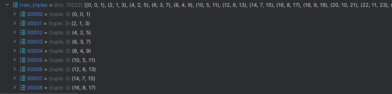
获取索引三元组
train_triples = read_triple(os.path.join(args.data_path, 'train.txt'), entity2id, relation2id)
def read_triple(file_path, entity2id, relation2id):
    '''
    Read triples and map them into ids.
    '''
    triples = []
    with open(file_path) as fin:
        # 打开文件
        for line in fin:
            # 形成索引三元组
            h, r, t = line.strip().split('\t')
            # 全部转换成索引
            triples.append((entity2id[h], relation2id[r], entity2id[t]))
    return triples
数据加载器
        # 设置数据加载器
        train_dataloader_head = DataLoader(
            TrainDataset(train_triples, nentity, nrelation, args.negative_sample_size, 'head-batch',args),
            batch_size=args.batch_size,
            shuffle=True,
            num_workers=max(1, args.cpu_num//2),
            collate_fn=TrainDataset.collate_fn,
            drop_last=True
        )

class TrainDataset(Dataset):
    def __init__(self, triples, nentity, nrelation, negative_sample_size, mode,args):
        # 存储三元组长度
        self.len = len(triples)
        # 存储三元组
        self.triples = triples
        # 创建三元组元组
        self.triple_set = set(triples)
        # 存储实体数量
        self.nentity = nentity
        # 存储关系数量
        self.nrelation = nrelation
        # 负样本尺寸
        self.negative_sample_size = negative_sample_size
        # 存储推断模式
        self.mode = mode
        # 计算三元组的频率
        self.count = self.count_frequency(triples)
        # 取得头实体和尾实体的真实值
        self.true_head, self.true_tail = self.get_true_head_and_tail(self.triples)

        # 存储训练参数
        self.args = args

    def __len__(self):
        return self.len

    def __getitem__(self, idx):
        # 根据索引获取正样本
        positive_sample = self.triples[idx]
        # 获取三元组
        head, relation, tail = positive_sample
        # 计算样本权重
        subsampling_weight = self.count[(head, relation)] + self.count[(tail, -relation-1)]
        subsampling_weight = torch.sqrt(1 / torch.Tensor([subsampling_weight]))
        # 数据格式转换
        positive_sample = torch.LongTensor(positive_sample)

        # 根据采样模式进行采样
        # 均匀随机采样
        if self.args.sample_method=='uni':
            # 负样本列表
            negative_sample_list = []
            # 负样本数量计数
            negative_sample_size = 0
            while negative_sample_size < self.negative_sample_size:
                # 生成self.negative_sample_size * 2个随机整数,这些整数的范围是从0到self.nentity(不包括self.nentity)
                negative_sample = np.random.randint(self.nentity, size=self.negative_sample_size*2)
                # 推断头实体
                if self.mode == 'head-batch':
                    # 从negative_sample这组随机数中选出,不是真实头实体索引对应的数字
                    mask = np.in1d(
                        negative_sample,
                        self.true_head[(relation, tail)],
                        # 元素唯一,可以提高效率
                        assume_unique=True,
                        # 数据反转
                        invert=True
                    )
                elif self.mode == 'tail-batch':
                    # 同理
                    mask = np.in1d(
                        negative_sample,
                        self.true_tail[(head, relation)],
                        assume_unique=True,
                        invert=True
                    )
                else:
                    raise ValueError('Training batch mode %s not supported' % self.mode)
                # 负样本数组
                negative_sample = negative_sample[mask]
                # 添加负样本数组
                negative_sample_list.append(negative_sample)
                # 计数
                negative_sample_size += negative_sample.size
            # 通过concat和切片获取负样本数组,
            negative_sample = np.concatenate(negative_sample_list)[:self.negative_sample_size]
            # 数据类型转换
            negative_sample = torch.LongTensor(negative_sample)
        # gumbel采样这是重点
        elif self.args.sample_method=='gumbel':
            # [self.nentity]指定张量形状
            mask = torch.ones([self.nentity], dtype=torch.float32,requires_grad=False)
            if self.mode == 'head-batch':
                # 获取标签
                label = self.true_head[(relation, tail)]
                # 标签近乎置零
                mask[label] = 1e-38
            elif self.mode == 'tail-batch':
                label = self.true_tail[(head, relation)]
                mask[label] = 1e-38
            # 只需转出掩码矩阵即可
            negative_sample = None


            ##################
        return positive_sample, negative_sample, subsampling_weight, mask,self.mode,self.args.sample_method

    @staticmethod
    def collate_fn(data):
        positive_sample = torch.stack([_[0] for _ in data], dim=0)
        if data[0][5]=='uni':
            negative_sample = torch.stack([_[1] for _ in data], dim=0)
            mask = None

        elif data[0][5]=='gumbel':
            mask = torch.stack([_[3] for _ in data], dim=0)
            negative_sample = None
        subsample_weight = torch.cat([_[2] for _ in data], dim=0)

        mode = data[0][4]
        return positive_sample, negative_sample, subsample_weight,mask, mode

    @staticmethod
    def count_frequency(triples, start=4):
        #对部分三元组(如(head, relation)或(relation, tail))的频率进行统计,
        # 对于实现类似于word2vec的子采样(subsampling)机制至关重要。
        # 这种子采样方法有助于减少训练过程中的计算负担,并提高模型的泛化能力。
        '''
        Get frequency of a partial triple like (head, relation) or (relation, tail)
        The frequency will be used for subsampling like word2vec
        '''
        count = {}
        for head, relation, tail in triples:
            if (head, relation) not in count:
                count[(head, relation)] = start
            else:
                count[(head, relation)] += 1

            if (tail, -relation-1) not in count:
                count[(tail, -relation-1)] = start
            else:
                count[(tail, -relation-1)] += 1
        return count

    @staticmethod
    def get_true_head_and_tail(triples):
        '''
        Build a dictionary of true triples that will
        be used to filter these true triples for negative sampling
        '''

        true_head = {}
        true_tail = {}
        # 获取对应的 实体;每一个元组对应一个实体列表
        for head, relation, tail in triples:
            if (head, relation) not in true_tail:
                true_tail[(head, relation)] = []
            true_tail[(head, relation)].append(tail)
            if (relation, tail) not in true_head:
                true_head[(relation, tail)] = []
            true_head[(relation, tail)].append(head)
        # 对true_head字典进行遍历,把键值对应的列表->集合->列表去除重复元素,最后转为np.array
        for relation, tail in true_head:
            true_head[(relation, tail)] = np.array(list(set(true_head[(relation, tail)])))
        for head, relation in true_tail:
            true_tail[(head, relation)] = np.array(list(set(true_tail[(head, relation)])))

        return true_head, true_tail
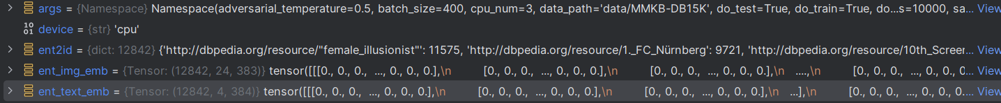
ent_text_emb,ent_img_emb嵌入
    ent_text_emb = torch.zeros([len(ent2id), 4, 384], device=device)
    ent_img_emb = torch.zeros([len(ent2id),24, 383], device=device)
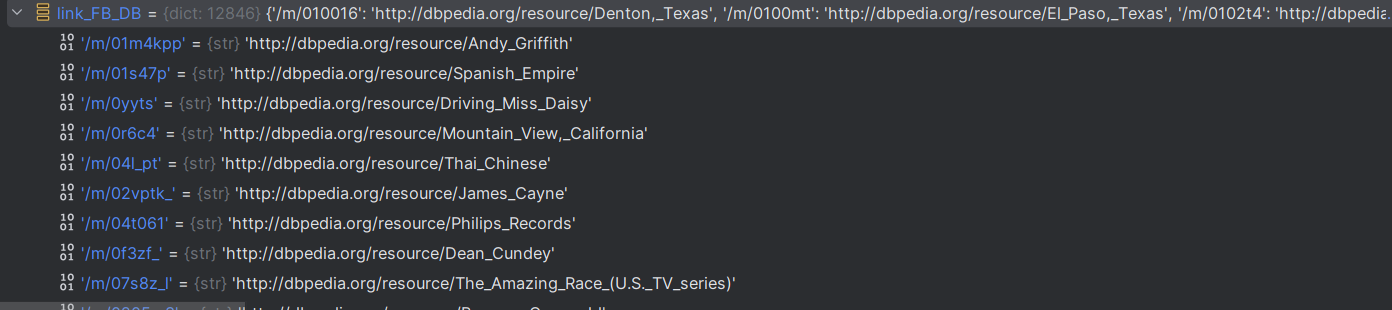
link_FB_DB
    # 这里没懂
    link_FB_DB = {}
    # 这里没懂
    ent_link_path_DB = 'data/MMKB-DB15K/DB15K_SameAsLink.txt'
    # 转换文件内容得到link_FB_DB
    with open(ent_link_path_DB) as fin:
        for line in fin:
            # 获取数据
            F,r,D,_ = line.strip().split(' ')
            # 切片去除特殊字符串
            link_FB_DB[F] = D[1:-1]
获取文本实体嵌入这段代码与前面的初始化嵌入相呼应,这里使用的嵌入流程就读取一个.h5文件,用ent2id去获取索引来进行嵌入。图像嵌入也是同理。
获取文本实体嵌入
# 计算KeyError的次数
    text_count = 0
    # 读取文本实体嵌入文件
    with h5py.File(text_path, 'r') as f:
        for k in f.keys():
            # 获取键值对应的数据,并且转换为np.array
            v = np.array(f[k])
            # 获取句子数量
            sentence_num = v.shape[0]
            try:
                # 实体名称
                name = 'http://dbpedia.org/resource/'+k
                # 因为ent_text_emb = torch.zeros([len(ent2id), 4, 384], device=device)限制了嵌入的维度
                # 长度大于4需要截断
                if sentence_num >=4:
                    ent_text_emb[ent2id[name]] = torch.from_numpy(v[:4])
                # 小于4全部嵌入
                else:
                    ent_text_emb[ent2id[name]][:sentence_num] = torch.from_numpy(v)
            except KeyError:
                text_count += 1

image_count = 0
    with h5py.File(image_path, 'r') as f:
        for k in f.keys():
            v = np.array(f[k])
            try:
                name = link_FB_DB['/m/'+k[2:]]
                ent_img_emb[ent2id[name]] = torch.from_numpy(v)

            except KeyError:
                image_count += 1

样本获取过程
    def __getitem__(self, idx):
        # 根据索引获取正样本
        positive_sample = self.triples[idx]
        # 获取三元组
        head, relation, tail = positive_sample
        # 计算样本权重
        subsampling_weight = self.count[(head, relation)] + self.count[(tail, -relation-1)]
        subsampling_weight = torch.sqrt(1 / torch.Tensor([subsampling_weight]))
        # 数据格式转换
        positive_sample = torch.LongTensor(positive_sample)

        # 根据采样模式进行采样
        # 均匀随机采样
        if self.args.sample_method=='uni':
            # 负样本列表
            negative_sample_list = []
            # 负样本数量计数
            negative_sample_size = 0
            while negative_sample_size < self.negative_sample_size:
                # 生成self.negative_sample_size * 2个随机整数,这些整数的范围是从0到self.nentity(不包括self.nentity)
                negative_sample = np.random.randint(self.nentity, size=self.negative_sample_size*2)
                # 推断头实体
                if self.mode == 'head-batch':
                    # 从negative_sample这组随机数中选出,不是真实头实体索引对应的数字
                    mask = np.in1d(
                        negative_sample,
                        self.true_head[(relation, tail)],
                        # 元素唯一,可以提高效率
                        assume_unique=True,
                        # 数据反转
                        invert=True
                    )
                elif self.mode == 'tail-batch':
                    # 同理
                    mask = np.in1d(
                        negative_sample,
                        self.true_tail[(head, relation)],
                        assume_unique=True,
                        invert=True
                    )
                else:
                    raise ValueError('Training batch mode %s not supported' % self.mode)
                # 负样本数组
                negative_sample = negative_sample[mask]
                # 添加负样本数组
                negative_sample_list.append(negative_sample)
                # 计数
                negative_sample_size += negative_sample.size
            # 通过concat和切片获取负样本数组,
            negative_sample = np.concatenate(negative_sample_list)[:self.negative_sample_size]
            # 数据类型转换
            negative_sample = torch.LongTensor(negative_sample)
        # gumbel采样这是重点
        elif self.args.sample_method=='gumbel':
            # [self.nentity]指定张量形状
            mask = torch.ones([self.nentity], dtype=torch.float32,requires_grad=False)
            if self.mode == 'head-batch':
                # 获取标签
                label = self.true_head[(relation, tail)]
                # 标签近乎置零
                mask[label] = 1e-38
            elif self.mode == 'tail-batch':
                label = self.true_tail[(head, relation)]
                mask[label] = 1e-38
            # 只需转出掩码矩阵即可
            negative_sample = None


            ##################
        return positive_sample, negative_sample, subsampling_weight, mask,self.mode,self.args.sample_method
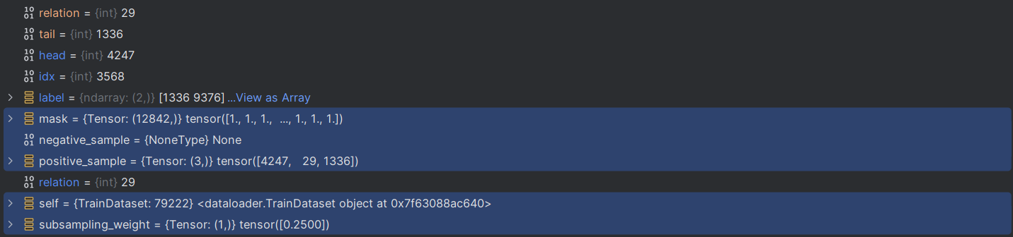
一次数据取出来之后是这样的,400是批量大小


 浙公网安备 33010602011771号