第4课：Unsupervised Learning-非监督式集群分析

目录

一.K-Means

1. K-Means理论

 2.代码

二 Hierarchical Clustering

1.理论

2.代码

三 Soft Clustering-Mixture models

1.理论

 2.代码

---

一.K-Means

简而言之就是分类问题。

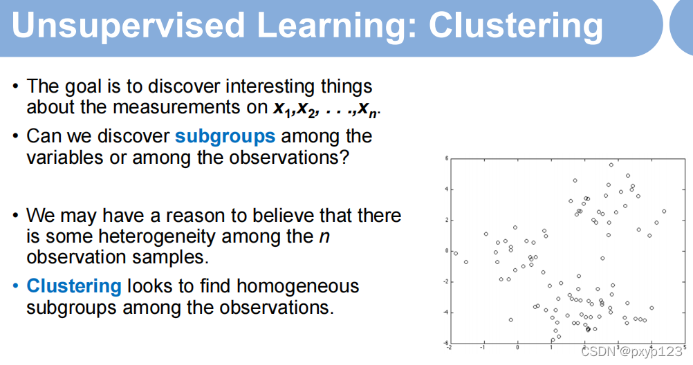
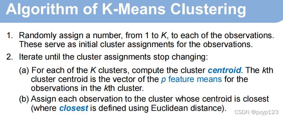
1. K-Means理论

自己划分K个分类集合，每个集合不相交，所有集合加起来是全集。一般使用欧几里得距离分集。

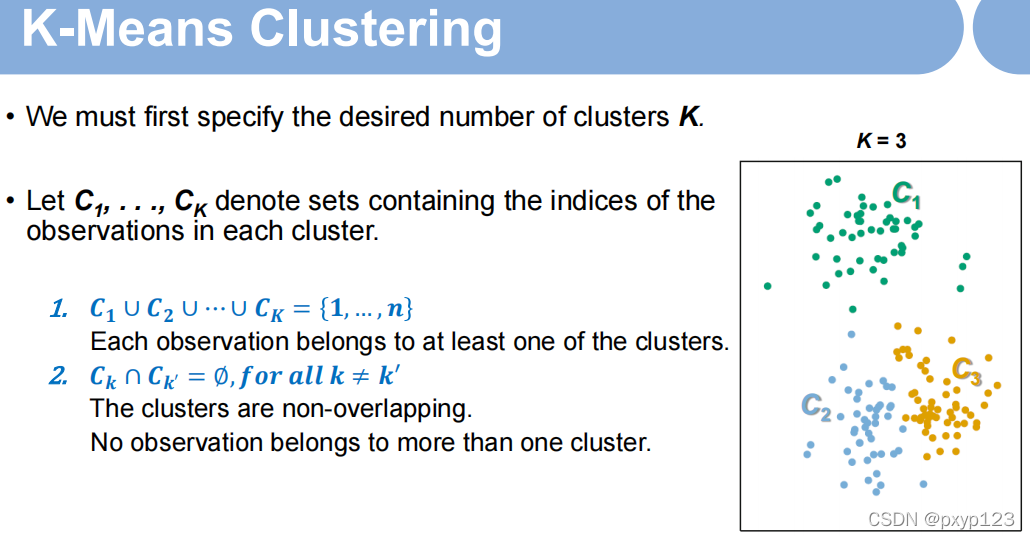
 K-Means的相似度判别准则：

 2.代码

使用的是Matlab 2018b，使用matlab自带的鸢尾花数据集。

%% An exercise of K-means clustering
clear, close all

%% Fisher's Iris dataset
% 50 samples from each of three species of?Iris
% Four features were measured from each sample: the length and the width of the sepals and petals (in cm)
load fisheriris
figure,
plot3(meas(:,1),meas(:,2),meas(:,3),'k.','markersize',10) % only plot first 3 features 
grid on
xlabel('feature 1'),ylabel('feature 2'),zlabel('feature 3')

%% Perform K-means clustering on the dataset
K=3;
[ind,C,sumd] = kmeans(meas,K);

figure, hold on
plot3(meas(ind==1,1),meas(ind==1,2),meas(ind==1,3),'r.','markersize',10) % only plot first 3 features
plot3(C(1,1),C(1,2),C(1,3),'kx','markersize',20,'linewidth',3) % only plot first 3 features
plot3(meas(ind==2,1),meas(ind==2,2),meas(ind==2,3),'g.','markersize',10) % only plot first 3 features 
plot3(C(2,1),C(2,2),C(2,3),'kx','markersize',20,'linewidth',3) % only plot first 3 features
plot3(meas(ind==3,1),meas(ind==3,2),meas(ind==3,3),'b.','markersize',10) % only plot first 3 features 
plot3(C(3,1),C(3,2),C(3,3),'kx','markersize',20,'linewidth',3) % only plot first 3 features
view(3)

grid on
xlabel('feature 1'),ylabel('feature 2'),zlabel('feature 3')
title(['Total sum of dist = ', num2str(sum(sumd))])

%% Perform K-means clustering with 20 replicates and parallel computing
opts = statset('Display','final','UseParallel',1);
%means：方法； 3是K； Maxlter：最大迭代次数； Replicates：迭代20次
[ind,C,sumd] = kmeans(meas,3,'MaxIter',10000,...
   'Replicates',20,'Options',opts);

figure, hold on
plot3(meas(ind==1,1),meas(ind==1,2),meas(ind==1,3),'r.','markersize',10) % only plot first 3 features
plot3(C(1,1),C(1,2),C(1,3),'kx','markersize',20,'linewidth',3) % only plot first 3 features
plot3(meas(ind==2,1),meas(ind==2,2),meas(ind==2,3),'g.','markersize',10) % only plot first 3 features 
plot3(C(2,1),C(2,2),C(2,3),'kx','markersize',20,'linewidth',3) % only plot first 3 features
plot3(meas(ind==3,1),meas(ind==3,2),meas(ind==3,3),'b.','markersize',10) % only plot first 3 features 
plot3(C(3,1),C(3,2),C(3,3),'kx','markersize',20,'linewidth',3) % only plot first 3 features
view(3)

grid on
xlabel('feature 1'),ylabel('feature 2'),zlabel('feature 3')
title(['Total sum of dist = ', num2str(sum(sumd))])

二 Hierarchical Clustering

1.理论

相当于自动划分K的集合，看你的坐标轴从哪里开始分割，即下图右边虚线位置（图中所示划分了2个）

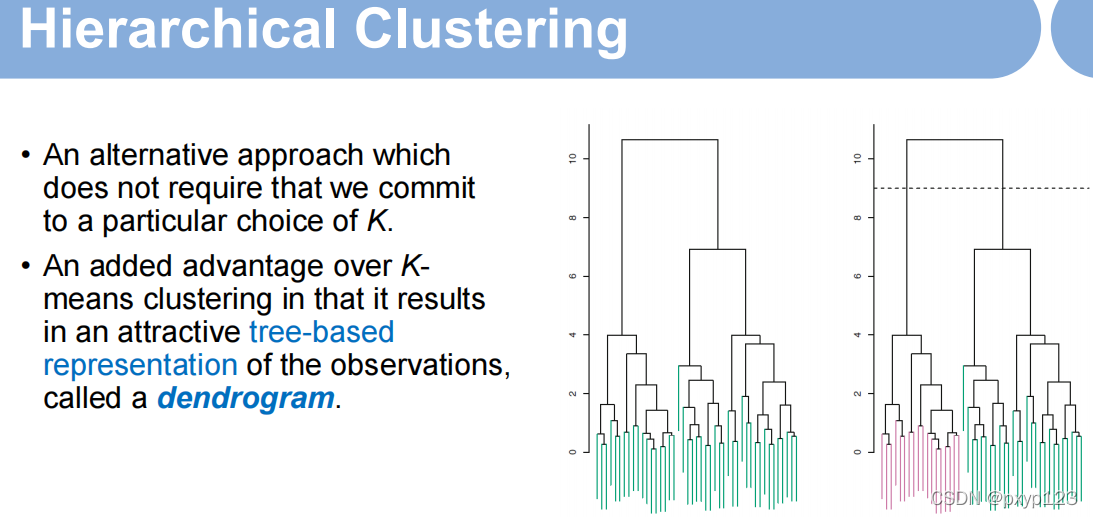
 dendrogram就是上图右边所示的树图，按照相似度两两划分。解释如下：

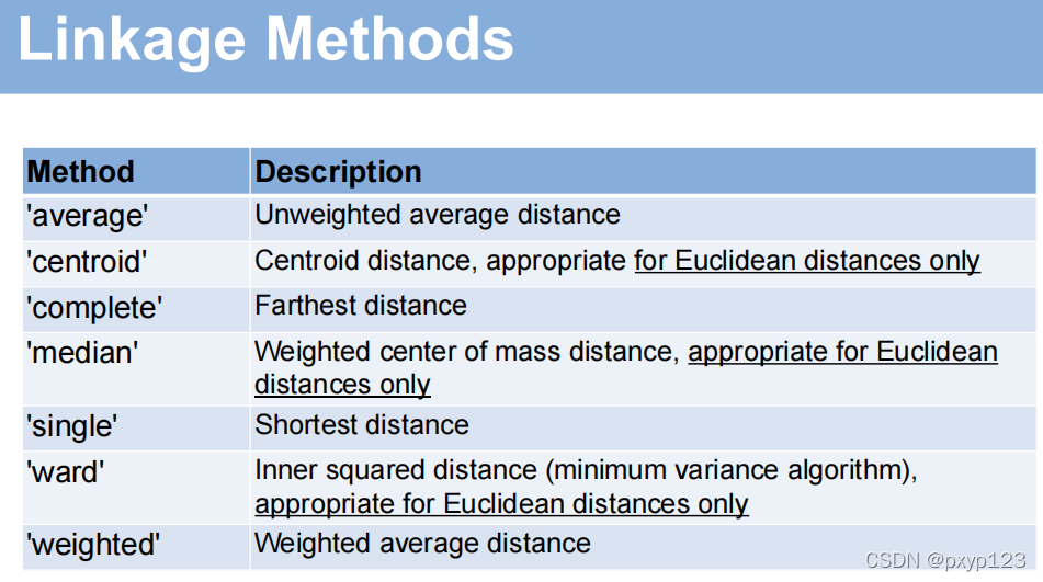
 linkage是matlab中的分类函数，划分标准如下， dendrogram是画出树图：

2.代码

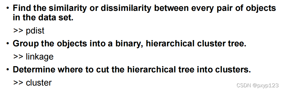
分三步：

 数据集在这里。ML-4，集群学习的数据集-Matlab文档类资源-CSDN下载ML-4，集群学习的数据集CancerMicroarrayProjectNCI60isa更多下载资源、学习资料请访问CSDN下载频道.https://download.csdn.net/download/pxyp123/84359093

%% An exercise of hirarchical clustering

clear, close all

%% NCI60 Cancer Cell Line Data
[numdata,CellLine,raw]=xlsread('NCI60data.csv');
numdata(1,:)=[]; % remove the first row in num，不导入第一行

%% standardize the variables to have mean zero and standard deviation one.
% 标准化：使得均值为0，标准差为1
Z=zscore(numdata);

%% Find the similarity or dissimilarity between every pair of objects in the data set.
% 64*63/2=2016
D=pdist(Z,'euclidean');  % D is a 1-by-(M*(M-1)/2) row vector. M is the number of observations.

%% Group the objects into a binary,?hierarchical?cluster?tree.
CT_complete=linkage(D,'complete');
figure,
%CT_complete:输入数据； 0：全部显示癌症种类（10，20就是显示十个，二十个）
%Labels：标签，不给标签会默认使用数字（1，2，...）分类； Orientation：树状图的走向（左右或者上下）
%outperm_complete：给出重新排序后的标签（癌症种类），按照相似度排序
[H,T,outperm_complete]=dendrogram(CT_complete,0,'Labels',CellLine,'Orientation','top');
set(gca,'XTickLabelRotation',90)
title('Complete Linkage')

CT_average=linkage(D,'average');
figure,
[H,T,outperm_average]=dendrogram(CT_average,0,'Labels',CellLine,'Orientation','top');
set(gca,'XTickLabelRotation',90)
title('Average Linkage')

CT_single=linkage(D,'single');
figure,
[H,T,outperm_single]=dendrogram(CT_single,0,'Labels',CellLine,'Orientation','top');
set(gca,'XTickLabelRotation',90)
title('Single Linkage')

%% Determine where to cut the?hierarchical?tree into?clusters.
K=5; % number of clusters
Clabel = cluster(CT_complete,'maxclust',K);

%% Display the original and reordered hotmap
cmap=[zeros(5,1), linspace(1,0,5)',zeros(5,1) ; linspace(0,1,5)',zeros(5,2)];
cmap(6,:)=[];

figure, 
subplot(1,2,1),imagesc(Z(:,1:500)'),title('Original Hotmap (part)')
subplot(1,2,2),imagesc(Z(outperm_complete,1:500)'),title('Clustered Hotmap (part)')
colormap(cmap)

三 Soft Clustering-Mixture models

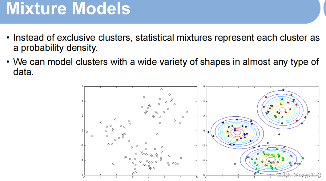
1.理论

引进统计的概念，以高斯模型为例。越靠近里面属于这个集合的几率就越高。每个集合的分布（可以直观理解为集合的宽和高）可以不一样。

假定xn属于第k个集合，高斯模型的均值和协方差已知的条件下，xn真正属于k集合的条件概率。如下图，Π1表示该点属于第一个集合的概率。如果有两个集合的概率相等，可以都选属于该集合。

 

 使用最大似然估计进行样本点的估计。不知道具体值时先猜测一个随机的值，然后一步一步进行迭代更新。

 2.代码

%% An exercise of Gaussian mixture model (GMM) for soft clustering
%% An example from MATLAB "Cluster Gaussian Mixture Data Using Soft Clustering"

clear, close all

%% Create simulated data from a mixture of two bivariate Gaussian distributions.
rng(0,'twister')  % For reproducibility
mu1 = [1 2]; %第一个均值
sigma1 = [3 .2; .2 2];%第一个协方差
mu2 = [-1 -2];
sigma2 = [2 0; 0 1];
X = [mvnrnd(mu1,sigma1,200); mvnrnd(mu2,sigma2,100)];

figure, hold on
plot(X(:,1),X(:,2),'k.','markersize',10) % only plot first 3 features 
xlabel('feature 1'),ylabel('feature 2')

%% Fit a two-component Gaussian mixture model (GMM)
K=2; % number of clusters
gm = fitgmdist(X,K);
for i=1:K
    [Xt,Yt,Z]=plot_2D_gauss(gm.mu(i,:),gm.Sigma(:,:,i));
    contour(Xt,Yt,Z,7,'linewidth',1);
    colormap(hsv)
end

%% Estimate component-member posterior probabilities for all data points using the fitted GMM gm.
P = posterior(gm,X);

n = size(X,1);
[~,order] = sort(P(:,1));

figure
plot(1:n,P(order,1),'r-',1:n,P(order,2),'b-')
legend({'Cluster 1', 'Cluster 2'})
ylabel('Cluster Membership Score')
xlabel('Point Ranking')
title('GMM with Full Unshared Covariances')

%% Plot the data and assign clusters by maximum posterior probability. 
% Identify points that could be in either cluster.
threshold = [0.4 0.6];

ind = cluster(gm,X);
indBoth = find(P(:,1)>=threshold(1) & P(:,1)<=threshold(2)); 
numInBoth = numel(indBoth)

figure
gscatter(X(:,1),X(:,2),ind,'rb','+o',5)
hold on
plot(X(indBoth,1),X(indBoth,2),'ko','MarkerSize',10)
legend({'Cluster 1','Cluster 2','Both Clusters'},'Location','SouthEast')
title('Scatter Plot - GMM with Full Unshared Covariances')

其中， gm = fitgmdist(X,K)可以查看你的拟合结果的均值和协方差。可以在工作区间查看。

gm = fitgmdist(X,K)
%Fit a two-component Gaussian mixture model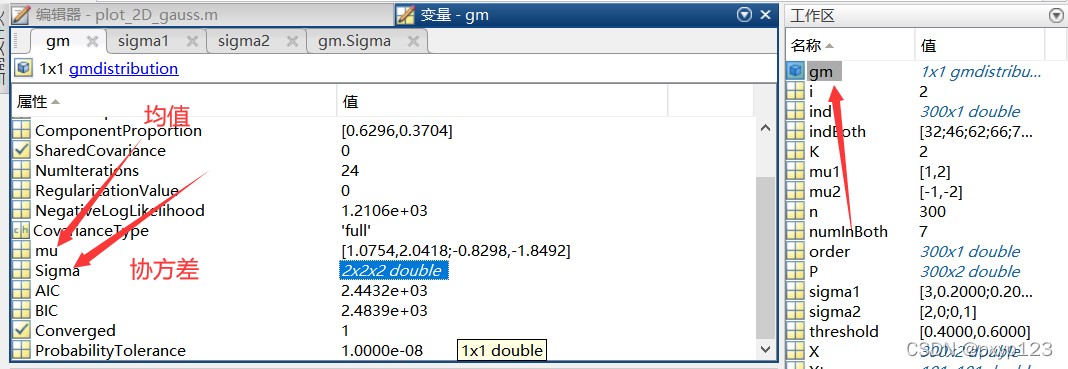

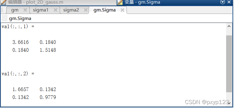
 以下是实际的均值和协方差，可以看到结果差不多。

 P = posterior(gm,X); 查看和集合的拟合情况

 P = posterior(gm,X); 
%Estimate component-member posterior probabilities for all data points

 ind = cluster(gm,X)：对样本点做分类处理；同时对于区间再0.4-0.6的样本点，可以让他们同时属于两个集合。

%Assign clusters by maximum posterior probability
ind = cluster(gm,X);

% Identify points that could be in either cluster.
threshold = [0.4 0.6];
indBoth = find(P(:,1)>=threshold(1) & P(:,1)<=threshold(2)); 
numInBoth = numel(indBoth)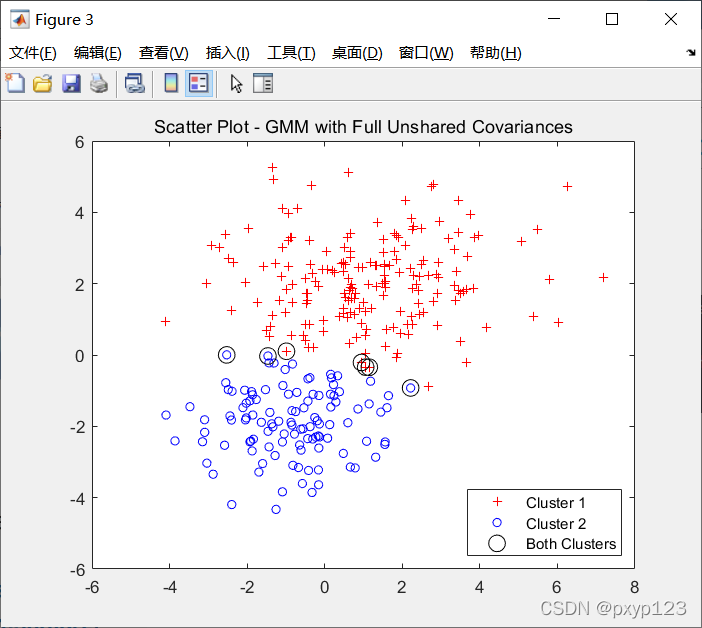

其中的 plot_2D_gauss函数如下。

function [Xt,Yt,Z]=plot_2D_gauss(mu,Sigma)
%% Plots the pdf of a 2D Gaussian as a surface
% From 'A first course in Machine Learning'


% Create a dense grid of points at which to evaluate the pdf
[Xt,Yt] = meshgrid(-5:0.1:5,-5:0.1:5);

% Compute the constant
const = 1/((2*pi)*sqrt(det(Sigma)));

% Evaluate the pdf at each grid point
Z = zeros(size(Xt));

for i = 1:numel(Xt)
    ve = [Xt(i);Yt(i)];    
    Z(i) = const * exp(-0.5 * (ve-mu')' * inv(Sigma)*(ve-mu'));%+...
%         0.7*const*exp(-0.5 * (ve-mu2)' * inv(Sigma)*(ve-mu2));
end

%% Create the contour plot and make it look nice
% figure
% contour(Xt,Yt,Z,7,'linewidth',1)
% colormap(gray)
% xlabel('$w_1$','interpreter','latex','fontsize',30)
% ylabel('$w_2$','interpreter','latex','fontsize',30)