线性回归

1 简单练习

输出一个5*5的单位矩阵

A = eye(5);

ans =

     1     0     0     0     0
     0     1     0     0     0
     0     0     1     0     0
     0     0     0     1     0
     0     0     0     0     1

2 单变量的线性回归

整个2的部分需要根据城市人口数量，预测开小吃店的利润 数据在ex1data1.txt里，第一列是城市人口数量，第二列是该城市小吃店利润。

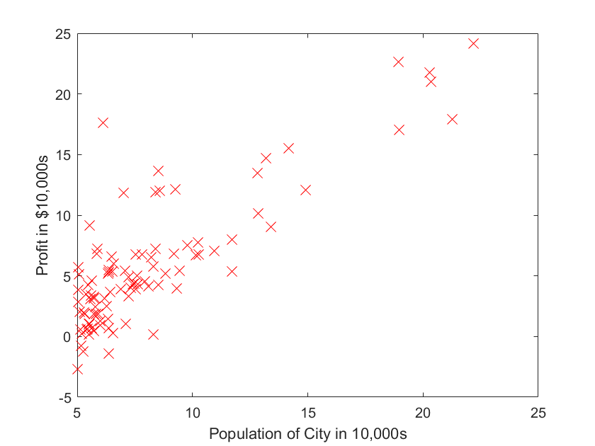
2.1 Plotting the Data

读入数据，然后展示数据

fprintf('Plotting Data ...\n')
data = load('ex1data1.txt');
x= data(:, 1); 
y =data(:, 2);
m = length(y); % number of training examples



plot(x, y, 'rx', 'MarkerSize', 10); % Plot the data 
%绘制图形：rx代表图形中标记的点为红色的x，数字10表示标记的大小。
ylabel('Profit in $10,000s'); % Set the y−axis label 
xlabel('Population of City in 10,000s'); % Set the x−axis label 

fprintf('Program paused. Press enter to continue.\n');
pause;

2.2 梯度下降

这个部分你需要在现有数据集上，训练线性回归的参数θ

2.2.1 约定公式

线性回归的目的是最小化成本函数

\[\begin{aligned} J(\theta) &=\frac{1}{2 m} \sum_{i=1}^{m}\left(h_{\theta}\left(x^{(i)}\right)-y^{(i)}\right)^{2} \end{aligned} \]

假设\(h_{\theta}(x)\)由线性模型给出

\[\begin{aligned} h_{\theta}(x) &=\theta^{T} X=\theta_{0}+\theta_{1} x_{1} \end{aligned} \]

梯度下降更新来最小化成本\(J{(\theta)}\):

\[\begin{aligned} \theta_{j}:=\theta_{j} &-\alpha \frac{1}{m} \sum_{i=1}^{m}\left(h_{\theta}\left(x^{(i)}\right)-y^{(i)}\right) x_{j}^{(i)} \end{aligned} \]

实现代码：

function J = computeCost(X, y, theta)
%COMPUTECOST Compute cost for linear regression
%   J = COMPUTECOST(X, y, theta) computes the cost of using theta as the
%   parameter for linear regression to fit the data points in X and y

% Initialize some useful values
m = length(y); % number of training examples

% You need to return the following variables correctly 
J = 0;

% ====================== YOUR CODE HERE ======================
% Instructions: Compute the cost of a particular choice of theta
%               You should set J to the cost.

%计算代价函数
J=sum((X*theta-y).^2)/(2*m);

% =========================================================================

end

2.2.2实现

数据前面已经读取完毕，我们要为加入一列x，用于更新\(\theta_{0}\)，然后我们将\(θ\)初始化为0，学习率初始化为0.01，迭代次数为1500次

X = [ones(m, 1), data(:,1)]; % Add a column of ones to x
theta = zeros(2, 1); % initialize fitting parameters
iterations = 1500;
alpha = 0.01;

2.2.3计算J(θ)

答案应该是32.07

J =

   32.0727

2.2.4 梯度下降

记住J(θ)的变量是θ，而不是X和y，意思是说，我们变化θ的值来使J(θ)变化，而不是变化X和y的值。 一个检查梯度下降是不是在正常运作的方式，是打印出每一步J(θ)的值，看他是不是一直都在减小，并且最后收敛至一个稳定的值。 θ最后的结果会用来预测小吃店在35000及70000人城市规模的利润。

function [theta, J_history] = gradientDescent(X, y, theta, alpha, num_iters)
%GRADIENTDESCENT Performs gradient descent to learn theta
%   theta = GRADIENTDESCENT(X, y, theta, alpha, num_iters) updates theta by 
%   taking num_iters gradient steps with learning rate alpha

% Initialize some useful values
m = length(y); % number of training examples
J_history = zeros(num_iters, 1);

for iter = 1:num_iters

    % ====================== YOUR CODE HERE ======================
    % Instructions: Perform a single gradient step on the parameter vector
    %               theta. 
    %
    % Hint: While debugging, it can be useful to print out the values
    %       of the cost function (computeCost) and gradient here.
    %


    x=X(:,2);
    theta0=theta(1);
    theta1=theta(2);
    
    theta0=theta0-alpha/m*sum(X*theta-y);
    theta1=theta1-alpha/m*sum((X*theta-y).*x);
    
    theta=[theta0;theta1];


    % ============================================================

    % Save the cost J in every iteration    
    J_history(iter) = computeCost(X, y, theta);

end

end

现在让我们运行梯度下降算法来将我们的参数θ适合于训练集。

theta = gradientDescent(X, y, theta, alpha, iterations);

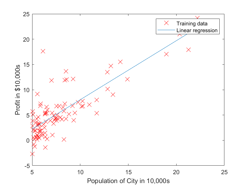
原始数据以及拟合的直线

% Plot the linear fit
hold on; % keep previous plot visible
plot(X(:,2), X*theta, '-')
legend('Training data', 'Linear regression')
hold off % don't overlay any more plots on this figure

预测35000和70000城市规模的小吃摊利润

% Predict values for population sizes of 35,000 and 70,000
predict1 = [1, 3.5] *theta;
fprintf('For population = 35,000, we predict a profit of %f\n',...
    predict1*10000);
predict2 = [1, 7] * theta;
fprintf('For population = 70,000, we predict a profit of %f\n',...
    predict2*10000);

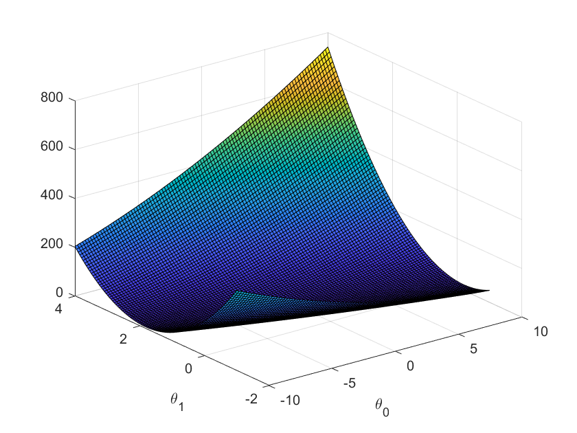
2.4 可视化J(θ)

此步可以便于你理解J(θ)以及梯度下降。 三维图显示了θ0和θ1与J(θ)的对应关系，J(θ)是一个碗状的图形，并且有全局最小值。这个最小值就是θ0和θ1的最优解。梯度下降的每一步都会更接近这个最小值。

fprintf('Visualizing J(theta_0, theta_1) ...\n')
% Grid over which we will calculate J
theta0_vals = linspace(-10, 10, 100);
theta1_vals = linspace(-1, 4, 100);

% initialize J_vals to a matrix of 0's
J_vals = zeros(length(theta0_vals), length(theta1_vals));

% Fill out J_vals
for i = 1:length(theta0_vals)
    for j = 1:length(theta1_vals)
	  t = [theta0_vals(i); theta1_vals(j)];
	  J_vals(i,j) = computeCost(X, y, t);
    end
end

J_vals = J_vals';
% Surface plot
figure;
surf(theta0_vals, theta1_vals, J_vals)%曲面图
xlabel('\theta_0'); 
ylabel('\theta_1');

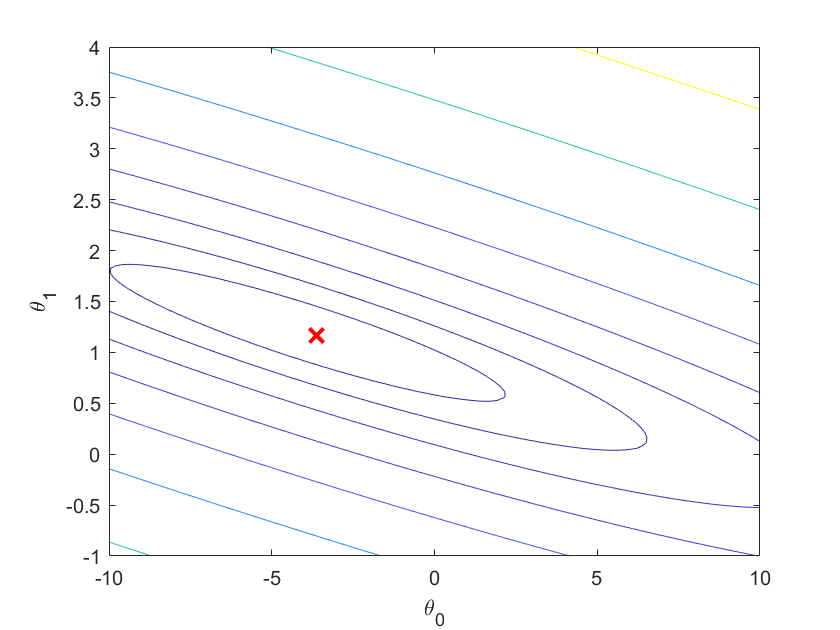
% Contour plot
figure;
% Plot J_vals as 15 contours spaced logarithmically between 0.01 and 100
contour(theta0_vals, theta1_vals, J_vals, logspace(-2, 3, 20))%矩阵的等高线图
%（logspace函数和linspace函数类似，此处作用生成将区间[10-2,103]等分20份的1*20矩阵）
xlabel('\theta_0');
ylabel('\theta_1');
hold on;
plot(theta(1), theta(2), 'rx', 'MarkerSize', 10, 'LineWidth', 2);

结果如下：

• 从图中可看出代价函数值*J*(θ)有全局最优解（最低点）

• 可以看出我们求出的最优参数θ所对应的代价值，正好位于等高线图最低的位置

  

  

2.5完整代码

2.5.1 主代码

A = eye(5);

fprintf('Plotting Data ...\n')
data = load('ex1data1.txt');
x= data(:, 1); % 表示data矩阵的第一列所有行， 并且取转置
y =data(:, 2);
m = length(y); % number of training examples



plot(x, y, 'rx', 'MarkerSize', 10); % Plot the data 
%绘制图形：rx代表图形中标记的点为红色的x，数字10表示标记的大小。
ylabel('Profit in $10,000s'); % Set the y−axis label 
xlabel('Population of City in 10,000s'); % Set the x−axis label 

fprintf('Program paused. Press enter to continue.\n');
pause;


X = [ones(m, 1), data(:,1)]; % Add a column of ones to x
theta = zeros(2, 1); % initialize fitting parameters
iterations = 1500;
alpha = 0.01;

fprintf('\nTesting the cost function ...\n')
% compute and display initial cost
J = computeCost(X, y, theta);
fprintf('With theta = [0 ; 0]\nCost computed = %f\n', J);
fprintf('Expected cost value (approx) 32.07\n');

fprintf('Program paused. Press enter to continue.\n');
pause;

fprintf('\nRunning Gradient Descent ...\n')
% run gradient descent
theta = gradientDescent(X, y, theta, alpha, iterations);

% print theta to screen
fprintf('Theta found by gradient descent:\n');
fprintf('%f\n', theta);
fprintf('Expected theta values (approx)\n');
fprintf(' -3.6303\n  1.1664\n\n');

% Plot the linear fit
hold on; % keep previous plot visible
plot(X(:,2), X*theta, '-')
legend('Training data', 'Linear regression')
hold off % don't overlay any more plots on this figure

% Predict values for population sizes of 35,000 and 70,000
predict1 = [1, 3.5] *theta;
fprintf('For population = 35,000, we predict a profit of %f\n',...
    predict1*10000);
predict2 = [1, 7] * theta;
fprintf('For population = 70,000, we predict a profit of %f\n',...
    predict2*10000);

fprintf('Program paused. Press enter to continue.\n');
pause;

fprintf('Visualizing J(theta_0, theta_1) ...\n')
% Grid over which we will calculate J
theta0_vals = linspace(-10, 10, 100);
theta1_vals = linspace(-1, 4, 100);

% initialize J_vals to a matrix of 0's
J_vals = zeros(length(theta0_vals), length(theta1_vals));

% Fill out J_vals
for i = 1:length(theta0_vals)
    for j = 1:length(theta1_vals)
	  t = [theta0_vals(i); theta1_vals(j)];
	  J_vals(i,j) = computeCost(X, y, t);
    end
end

J_vals = J_vals';
% Surface plot
figure;
surf(theta0_vals, theta1_vals, J_vals)%曲面图
xlabel('\theta_0'); 
ylabel('\theta_1');

% Contour plot
figure;
% Plot J_vals as 15 contours spaced logarithmically between 0.01 and 100
contour(theta0_vals, theta1_vals, J_vals, logspace(-2, 3, 20))%矩阵的等高线图
%（logspace函数和linspace函数类似，此处作用生成将区间[10-2,103]等分20份的1*20矩阵）
xlabel('\theta_0');
ylabel('\theta_1');
hold on;
plot(theta(1), theta(2), 'rx', 'MarkerSize', 10, 'LineWidth', 2);

2.5.2 求梯度代码

function [theta, J_history] = gradientDescent(X, y, theta, alpha, num_iters)
%GRADIENTDESCENT Performs gradient descent to learn theta
%   theta = GRADIENTDESCENT(X, y, theta, alpha, num_iters) updates theta by 
%   taking num_iters gradient steps with learning rate alpha

% Initialize some useful values
m = length(y); % number of training examples
J_history = zeros(num_iters, 1);

for iter = 1:num_iters

    % ====================== YOUR CODE HERE ======================
    % Instructions: Perform a single gradient step on the parameter vector
    %               theta. 
    %
    % Hint: While debugging, it can be useful to print out the values
    %       of the cost function (computeCost) and gradient here.
    %


    x=X(:,2);
    theta0=theta(1);
    theta1=theta(2);
    
    theta0=theta0-alpha/m*sum(X*theta-y);
    theta1=theta1-alpha/m*sum((X*theta-y).*x);
    
    theta=[theta0;theta1];


    % ============================================================

    % Save the cost J in every iteration    
    J_history(iter) = computeCost(X, y, theta);

end

end

2.5.3 计算代价函数

function J = computeCost(X, y, theta)
%COMPUTECOST Compute cost for linear regression
%   J = COMPUTECOST(X, y, theta) computes the cost of using theta as the
%   parameter for linear regression to fit the data points in X and y

% Initialize some useful values
m = length(y); % number of training examples

% You need to return the following variables correctly 
J = 0;

% ====================== YOUR CODE HERE ======================
% Instructions: Compute the cost of a particular choice of theta
%               You should set J to the cost.

%计算代价函数
J=sum((X*theta-y).^2)/(2*m);



% =========================================================================

end

3 多变量线性回归

ex1data2.txt里的数据，第一列是房屋大小，第二列是卧室数量，第三列是房屋售价 根据已有数据，建立模型，预测房屋的售价

%%加载数据
data = load('ex1data2.txt');
X=data(:,1:2)
y=data(:,3)
m=length(y)

% Print out some data points
fprintf('First 10 examples from the dataset: \n');
fprintf(' x = [%.0f %.0f], y = %.0f \n', [X(1:10,:) y(1:10,:)]');

fprintf('Program paused. Press enter to continue.\n');
pause;

3.1 特征归一化

观察数据发现，size变量是bedrooms变量的1000倍大小,统一量级会让梯度下降收敛的更快。做法就是:将每类特征减去他的平均值后除以标准差

\[x_{n}=\frac{X_{n}-u_{n} }{s_{n} } \]

\(u_{n}\)是平均值，\(s_{n}\)是标准差

function [X_norm, mu, sigma] = featureNormalize(X)
%FEATURENORMALIZE Normalizes the features in X 
%   FEATURENORMALIZE(X) returns a normalized version of X where
%   the mean value of each feature is 0 and the standard deviation
%   is 1. This is often a good preprocessing step to do when
%   working with learning algorithms.

% You need to set these values correctly
X_norm = X;
mu = zeros(1, size(X, 2));
sigma = zeros(1, size(X, 2));

% ====================== YOUR CODE HERE ======================
% Instructions: First, for each feature dimension, compute the mean
%               of the feature and subtract it from the dataset,
%               storing the mean value in mu. Next, compute the 
%               standard deviation of each feature and divide
%               each feature by it's standard deviation, storing
%               the standard deviation in sigma. 
%
%               Note that X is a matrix where each column is a 
%               feature and each row is an example. You need 
%               to perform the normalization separately for 
%               each feature. 
%
% Hint: You might find the 'mean' and 'std' functions useful.
%       


mu=mean(X)
sigma=std(X)

for i = 1:size(X,2),
    X_norm(:,i) = (X(:,i) - mu(i)) / sigma(i);
end



% ============================================================

end

主函数运行：

% Scale features and set them to zero mean
fprintf('Normalizing Features ...\n');

[X mu sigma] = featureNormalize(X);

% Add intercept term to X
X = [ones(m, 1) X];

3.2 代价函数和梯度下降

代价函数：

function J = computeCostMulti(X, y, theta)
%COMPUTECOSTMULTI Compute cost for linear regression with multiple variables
%   J = COMPUTECOSTMULTI(X, y, theta) computes the cost of using theta as the
%   parameter for linear regression to fit the data points in X and y

% Initialize some useful values
m = length(y); % number of training examples

% You need to return the following variables correctly 
J = 0;

% ====================== YOUR CODE HERE ======================
% Instructions: Compute the cost of a particular choice of theta
%               You should set J to the cost.

J = ((X * theta - y)' * (X * theta - y))/(2*m);



% =========================================================================

end

梯度下降：

function [theta, J_history] = gradientDescentMulti(X, y, theta, alpha, num_iters)
%GRADIENTDESCENTMULTI Performs gradient descent to learn theta
%   theta = GRADIENTDESCENTMULTI(x, y, theta, alpha, num_iters) updates theta by
%   taking num_iters gradient steps with learning rate alpha

% Initialize some useful values
m = length(y); % number of training examples
J_history = zeros(num_iters, 1);

for iter = 1:num_iters

    % ====================== YOUR CODE HERE ======================
    % Instructions: Perform a single gradient step on the parameter vector
    %               theta. 
    %
    % Hint: While debugging, it can be useful to print out the values
    %       of the cost function (computeCostMulti) and gradient here.
    %
    
    theta = theta - alpha / m * X' * (X * theta - y);


    % ============================================================

    % Save the cost J in every iteration    
    J_history(iter) = computeCostMulti(X, y, theta);

end

end

3.3梯度下降的完整代码

%%加载数据
data = load('ex1data2.txt');
X=data(:,1:2)
y=data(:,3)
m=length(y)

% Print out some data points
fprintf('First 10 examples from the dataset: \n');
fprintf(' x = [%.0f %.0f], y = %.0f \n', [X(1:10,:) y(1:10,:)]');

fprintf('Program paused. Press enter to continue.\n');
pause;

% Scale features and set them to zero mean
fprintf('Normalizing Features ...\n');

[X mu sigma] = featureNormalize(X);

% Add intercept term to X
X = [ones(m, 1) X];


fprintf('Running gradient descent ...\n');

% Choose some alpha value
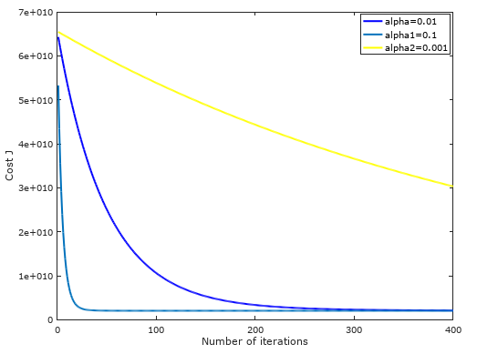
alpha = 0.01;
num_iters = 400;

% Init Theta and Run Gradient Descent 
theta = zeros(3, 1);
[theta, J_history] = gradientDescentMulti(X, y, theta, alpha, num_iters);

% Plot the convergence graph
figure;
plot(1:numel(J_history), J_history, '-b', 'LineWidth', 2);
xlabel('Number of iterations');
ylabel('Cost J');

% Display gradient descent's result
fprintf('Theta computed from gradient descent: \n');
fprintf(' %f \n', theta);
fprintf('\n');

% Estimate the price of a 1650 sq-ft, 3 br house
% ====================== YOUR CODE HERE ======================
% Recall that the first column of X is all-ones. Thus, it does
% not need to be normalized.
price = [1,1650,3]*theta; % You should change this

% ============================================================
fprintf(['Predicted price of a 1650 sq-ft, 3 br house ' ...
         '(using gradient descent):\n $%f\n'], price);

fprintf('Program paused. Press enter to continue.\n');
pause;

图片（选择学习速率）

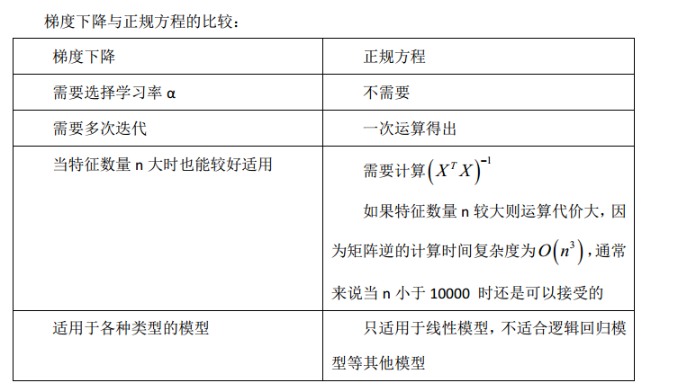
3.4 正规方程

正规方程是通过求解下面的方程来找出使得代价函数最小的参数的：\(\frac{\partial}{\partial \theta_{j} }J(\theta_{j})=0\) 。 假设我们的训练集特征矩阵为 X（包含了x0=1）并且我们的训练集结果为向量 y，则利用正规方程解出向量\((X^{T}X)^{-1}X^{T}y\) 。 上标T代表矩阵转置，上标-1 代表矩阵的逆。设矩阵\(A=X^{T}X\),则\(A^{-1}=(X^{T}X)^{-1}\)

function [theta] = normalEqn(X, y)
%NORMALEQN Computes the closed-form solution to linear regression 
%   NORMALEQN(X,y) computes the closed-form solution to linear 
%   regression using the normal equations.

theta = zeros(size(X, 2), 1);

% ====================== YOUR CODE HERE ======================
% Instructions: Complete the code to compute the closed form solution
%               to linear regression and put the result in theta.
%

% ---------------------- Sample Solution ----------------------

theta = pinv(X' * X) * X' * y


% -------------------------------------------------------------


% ============================================================

end

主函数完整代码

%% ================ Part 3: Normal Equations ================

fprintf('Solving with normal equations...\n');

% ====================== YOUR CODE HERE ======================
% Instructions: The following code computes the closed form 
%               solution for linear regression using the normal
%               equations. You should complete the code in 
%               normalEqn.m
%
%               After doing so, you should complete this code 
%               to predict the price of a 1650 sq-ft, 3 br house.
%

%% Load Data
data = csvread('ex1data2.txt');
X = data(:, 1:2);
y = data(:, 3);
m = length(y);

% Add intercept term to X
X = [ones(m, 1) X];

% Calculate the parameters from the normal equation
theta = normalEqn(X, y);

% Display normal equation's result
fprintf('Theta computed from the normal equations: \n');
fprintf(' %f \n', theta);
fprintf('\n');


% Estimate the price of a 1650 sq-ft, 3 br house
% ====================== YOUR CODE HERE ======================
price = [1,1650,3]*theta; % You should change this


% ============================================================

fprintf(['Predicted price of a 1650 sq-ft, 3 br house ' ...
         '(using normal equations):\n $%f\n'], price);