BP网络中的反向传播

本文的主要参考：How the backpropagation algorithm works

下面是BP网络的参数结构示意图

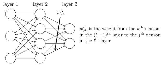
首先定义第l层网络第j个神经元的输出(activation)

为了表示简便，令

则有a^l_j=σ(z^l_j)，其中σ是激活函数

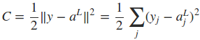
定义网络的cost function，其中的n是训练样本的个数。

下面主要介绍使用反向传播来求取cost function相对于权重w_ij和偏置项b_ij的导数。

显然，当输入已知时，cost function只是权值w和偏置项b的函数。这里为了方便推倒，首先计算出∂C/∂z^l_j，令

由于a^l_j=σ(z^l_j)，所以显然有

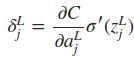
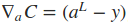
式中的L表示最后一层网络，即输出层。如果只考虑一个训练样本，则cost function可表示为

如果将输出层的所有输出看成一个列向量，则δ_j^L可以写成下式，Θ表示向量的点乘

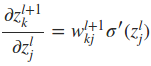
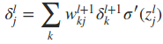
下面最关键的问题来了，如何同过δ^l+1求取δ^l。这里就用到了∂C/∂z^l_j这一重要的中间表达，推倒过程如下

 

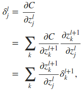
因此，最终有

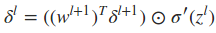
写成向量的形式为

利用与上面类似的推倒，可以得到

　

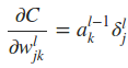
将上面重要的公式用矩阵乘法形式再表达一遍

　

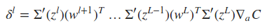
式中Σ^'(z^L)是主对角线上的元素为σ^'(z^L_j)的对角矩阵。求取了cost function相对于权重w_ij和偏置项b_ij的导数之后，便可以使用一些基于梯度的优化算法对网络的权值进行更新。下面是一个２输入２输出的一个BP网络的代码示例，实现的是对输入的每个元素进行逻辑取反操作。

import numpy as np

def tanh(x):
    return np.tanh(x)

def tanh_prime(x):
    x = np.tanh(x)
    return 1.0 - x ** 2

class Network(object):

    def __init__(self, sizes):
        self.num_layers = len(sizes)
        self.sizes = sizes
        # self.biases is a column vector
        # self.weights' structure is the same as in the book: http://neuralnetworksanddeeplearning.com/chap2.html
        self.biases = [np.random.randn(y, 1) for y in sizes[1:]]
        self.weights = [np.random.randn(y, x)
                        for x, y in zip(sizes[:-1], sizes[1:])]

    def feedforward(self, a):
        """Return the output of the network if "a" is input."""
        for b, w in zip(self.biases, self.weights):
            a = sigmoid(np.dot(w, a) + b)
        return a

    def update_mini_batch(self, mini_batch, learning_rate = 0.2):
        """Update the network's weights and biases by applying
        gradient descent using backpropagation to a single mini batch.
        The "mini_batch" is a list of tuples "(x, y)"."""
        nabla_b = [np.zeros(b.shape) for b in self.biases]
        nabla_w = [np.zeros(w.shape) for w in self.weights]
        
        # delta_nabla_b is dC/db, delta_nabla_w is dC/dw
        for x, y in mini_batch:
            delta_nabla_b, delta_nabla_w = self.backprop(x, y)
            nabla_b = [nb + dnb for nb, dnb in zip(nabla_b, delta_nabla_b)]
            nabla_w = [nw + dnw for nw, dnw in zip(nabla_w, delta_nabla_w)]
        self.weights = [w - (learning_rate/len(mini_batch)) * nw
                        for w, nw in zip(self.weights, nabla_w)]
        self.biases = [b - (learning_rate/len(mini_batch)) * nb
                       for b, nb in zip(self.biases, nabla_b)]

    def backprop(self, x, y):
        """Return a tuple ``(nabla_b, nabla_w)`` representing the
        gradient for the cost function C_x.  ``nabla_b`` and
        ``nabla_w`` are layer-by-layer lists of numpy arrays, similar
        to ``self.biases`` and ``self.weights``."""
        nabla_b = [np.zeros(b.shape) for b in self.biases]
        nabla_w = [np.zeros(w.shape) for w in self.weights]
        
        # feedforward
        activation = x
        activations = [x]   # list to store all the activations, layer by layer
        zs = []             # list to store all the z vectors, layer by layer
        
        # After this loop, activations = [a0, a1, ..., aL], zs = [z1, z2, ..., zL]
        for b, w in zip(self.biases, self.weights):
            z = np.dot(w, activation) + b
            zs.append(z)
            activation = sigmoid(z)
            activations.append(activation)
        
        # backward pass
        # delta = deltaL .* sigma'(zL)
        delta = self.cost_derivative(activations[-1], y) * \
                sigmoid_prime(zs[-1])
        
        # dC/dbL = delta
        # dC/dwL = deltaL * a(L-1)^T
        nabla_b[-1] = delta
        nabla_w[-1] = np.dot(delta, activations[-2].transpose())

        '''Note that the variable l in the loop below is used a little
        differently to the notation in Chapter 2 of the book. Here,
        l = 1 means the last layer of neurons, l = 2 is the
        second-last layer, and so on. It's a renumbering of the
        scheme in the book, used here to take advantage of the fact
        that Python can use negative indices in lists.'''
        # z = z(L-l+1), here, l start from 2, end with self.num_layers-1, namely, L-1
        # delta = delta(L-l+1) = w(L-l+2)^T * delta(L-l+2) .* z(L-l+1)
        # nabla_b[L-l+1] = delta(L-l+1)
        # nabla_w[L-l+1] = delta(L-l+1) * a(L-l)^T
        for l in xrange(2, self.num_layers):
            z = zs[-l]
            sp = sigmoid_prime(z)
            delta = np.dot(self.weights[-l + 1].transpose(), delta) * sp
            nabla_b[-l] = delta
            nabla_w[-l] = np.dot(delta, activations[-l - 1].transpose())
        return (nabla_b, nabla_w)

    def evaluate(self, test_data):
        """Return the number of test inputs for which the neural
        network outputs the correct result. Note that the neural
        network's output is assumed to be the index of whichever
        neuron in the final layer has the highest activation."""
        test_results = self.feedforward(test_data)
        return test_results

    def cost_derivative(self, output_activations, y):
        return (output_activations - y)

#### Miscellaneous functions
def sigmoid(z):
    return 1.0/(1.0 + np.exp(-z))

# derivative of the sigmoid function
def sigmoid_prime(z):
    return sigmoid(z) * (1 - sigmoid(z))

if __name__ == '__main__':

    nn = Network([2, 2, 2])

    X = np.array([[0, 0],
                  [0, 1],
                  [1, 0],
                  [1, 1]])

    y = np.array([[1, 1],
                  [1, 0],
                  [0, 1],
                  [0, 0]])
    
    for k in range(40000):
        if k % 10000 == 0:
            print 'epochs:', k
        # Randomly select a sample.
        i = np.random.randint(X.shape[0])
        nn.update_mini_batch(zip([np.atleast_2d(X[i]).T], [np.atleast_2d(y[i]).T]))

    for e in X:
        print(e, nn.evaluate(np.atleast_2d(e).T))

运行结果

epochs: 0
epochs: 10000
epochs: 20000
epochs: 30000
(array([0, 0]), array([[ 0.98389328],
       [ 0.97490859]]))
(array([0, 1]), array([[ 0.97694707],
       [ 0.01646559]]))
(array([1, 0]), array([[ 0.03149928],
       [ 0.97737158]]))
(array([1, 1]), array([[ 0.01347963],
       [ 0.02383405]]))