Jupyter —— 简单线性回归分析
Jupyter —— 简单线性回归分析
我们在前面的博客中已经介绍了什么是线性回归:回归分析
本片博客将从编程的角度介绍线性回归,这里主要分为使用 sklearn 库和非 sklearn 库来两种编程方式
sklearn 库线性回归分析
首先我们要读取本地数据
import numpy as np
import pandas as pd
from sklearn.linear_model import LinearRegression

# 读取 excel 表中数据
data = pd.read_excel("D:\code-file\conda\data\weights_heights.xls")
data.shape
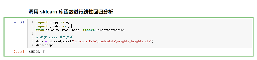
这里运行输出(25000,3)表示一共有 5000 组数据,每组有三个数据,对应 excel 表格中的三列
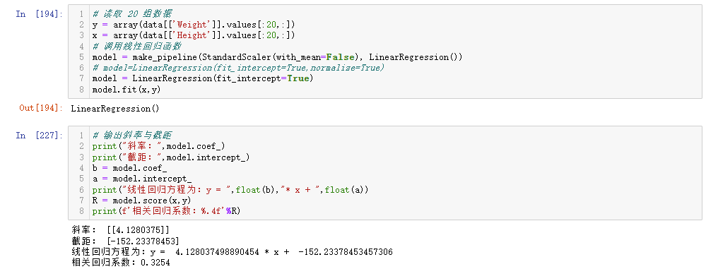
# 读取 20 组数据
y = array(data[['Weight']].values[:20,:])
x = array(data[['Height']].values[:20,:])
# 调用线性回归函数
model = LinearRegression(fit_intercept=True,normalize=True)
model.fit(x,y)
这里我们调用了 sklearn 的 linear_model 中的 LinearRegression() 函数,用于线性回归分析,LinearRegression() 函数共有两个参数:
-
fit_intercept 是否有截据,如果没有则直线过原点
-
normalize 是否将数据归一化
如果我们使用 normalize 参数会生成警告:
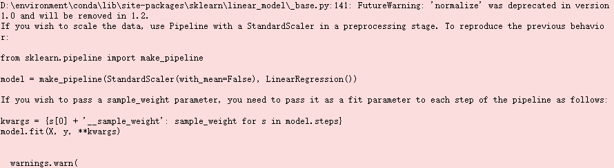
警告的意思大概是:
'normalize'在1.0版本中已弃用,将在1.2版本中移除,如果我们要继续使用,这里我们就要用以下方式进行代替:
from sklearn.pipeline import make_pipeline
from sklearn.preprocessing import StandardScaler
model = make_pipeline(StandardScaler(with_mean=False), LinearRegression())
# 输出斜率与截距
print("斜率:",model.coef_)
print("截距:",model.intercept_)
b = model.coef_
a = model.intercept_
y = b*x+a
print("线性回归方程为:y = ",float(b),"* x + ",float(a))
最后我们输出了线性回归方程并计算出 R$ ^2 $,
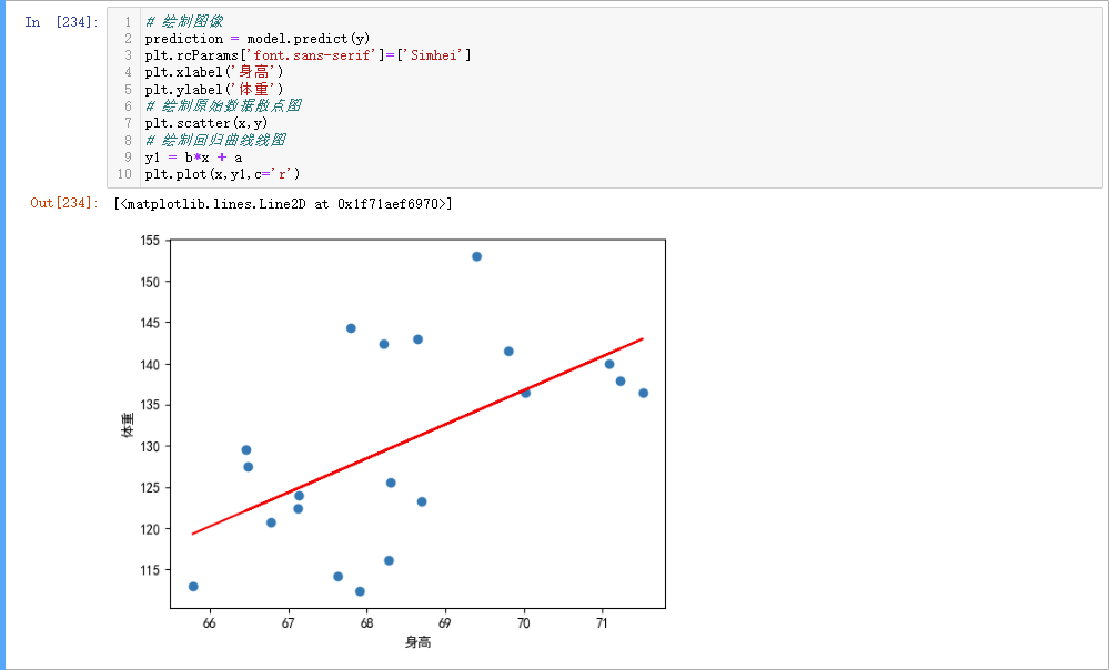
# 绘制图像
prediction = model.predict(y)
plt.xlabel('身高')
plt.ylabel('体重')
# 绘制原始数据散点图
plt.scatter(x,y)
# 绘制回归曲线线图
y1 = b*x + a
plt.plot(x,y1,c='r')
这里我们使用 matplotlib 库进行绘图,图中显示了原有散点分布和我们计算出来的回归方程对应的趋势曲线
如果我们图像中的汉字乱码,添加如下语句即可:
plt.rcParams['font.sans-serif']=['Simhei']
完整代码如下:
import numpy as np
import pandas as pd
import matplotlib.pyplot as plt
from numpy import array
from sklearn.pipeline import make_pipeline
from sklearn.preprocessing import StandardScaler
from sklearn.linear_model import LinearRegression

# 读取 excel 表中数据
data = pd.read_excel("D:\code-file\conda\data\weights_heights.xls",'weights_heights')
data.shape
# 读取 20 组数据
y = array(data[['Weight']].values[:20,:])
x = array(data[['Height']].values[:20,:])
# 调用线性回归函数
model = make_pipeline(StandardScaler(with_mean=False), LinearRegression())
# model=LinearRegression(fit_intercept=True,normalize=True)
model = LinearRegression(fit_intercept=True)
model.fit(x,y)
# 输出斜率与截距
print("斜率:",model.coef_)
print("截距:",model.intercept_)
b = model.coef_
a = model.intercept_
print("线性回归方程为:y = ",float(b),"* x + ",float(a))
R = model.score(x,y)
print(f'相关回归系数:%.4f'%R)
# 绘制图像
prediction = model.predict(y)
plt.rcParams['font.sans-serif']=['Simhei']
plt.xlabel('身高')
plt.ylabel('体重')
# 绘制原始数据散点图
plt.scatter(x,y)
# 绘制回归曲线线图
y1 = b*x + a
plt.plot(x,y1,c='r')
这里我们要是实现对不同数量的数据进行分析,我们可以直接修改其中一个参数,将数据数量从 [:20,:0] 修改为 [:x,:0] 即可
手写算法实现线性回归分析
首先调用对应的包,并从 excel 文件中读取数据:
# 调用包
import pandas as pd
import numpy as np
import matplotlib.pyplot as plt
import math
# 调用数据
data = pd.read_excel("D:\code-file\conda\data\weights_heights.xls",'weights_heights')
# 20组数据,需要更多数据修改参数就行
d = data.head(20)
d.shape
x=d["Height"]
y=d["Weight"]
我们这里先画出散点图,来确认我们是否成功读取了正确的数据:
# 绘制散点图图像
plt.scatter(x,y)
plt.axis([65,72,0,180])
plt.show()
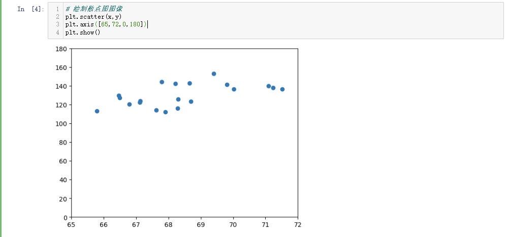
这里我们成功调用了数据,下面我们开始计算回归方程和相关系数,这里我们直接使用相关公式进行计算:
\[b = \frac{\sum^n_{i = 1}(x_i - \overline{x})(y_i - \bar{y})}{\sum_{i = 1}^n(x_i - \overline{x})^2}
\]
\[a = \bar{y} - b \overline{x}
\]
\[r = \frac{\sum^n_{i = 1}(x_i - \overline{x})(y_i - \bar{y})}{\sqrt{\sum_{i = 1}^n(x_i - \overline{x})^2}\sqrt{\sum_{i = 1}^n(y_i - \bar{y})^2}}
\]
# 利用公式求出 a、b、r
x_mean = np.mean(x)
y_mean = np.mean(y)
num = 0.0       #分子
d = 0.0         #分母
m = 0.0
for x_i, y_i in zip(x,y):
    num += (x_i - x_mean) * (y_i - y_mean)
    d  += (x_i - x_mean) ** 2
    m += (y_i - y_mean) ** 2
a = num/d
b = y_mean - a * x_mean
y1 = a * x + b
r=(num/((d** 0.5)*(m** 0.5)))**2
print("回归方程为:y = ",a,"x + ",b)
print("相关系数:",r)

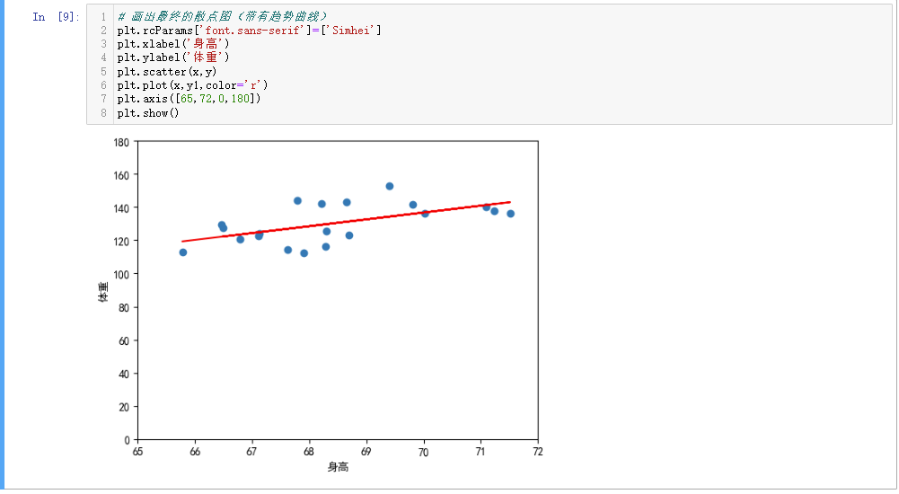
画出最终的散点图和趋势曲线:
# 画出最终的散点图(带有趋势曲线)
plt.rcParams['font.sans-serif']=['Simhei']
plt.xlabel('身高')
plt.ylabel('体重')
plt.scatter(x,y)
plt.plot(x,y1,color='r')
plt.axis([65,72,0,180])
plt.show()

 浙公网安备 33010602011771号