Analysis of Variance ANOVA versus T test 方差分析和T检验
Levels are different groupings within the same independent variable(factor).
Eg. if the independent variable is “eggs” the levels might be Non-Organic, Organic, and Free Range Organic.
Analysis of Variance ANOVA 方差分析
Goal
whether there is a significant difference between/among the levels of the independent variables.
Assumptions
- Independence of observations
- Normality the distributions of the residuals are normal
- Equality (or "homogeneity") of variances —the variance of data in groups should be the same.
Levels are different groupings within the same independent variable(factor).
Eg. if the independent variable is “eggs” the levels might be Non-Organic, Organic, and Free Range Organic.
Eg.
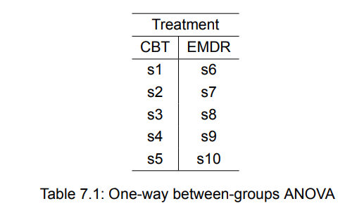
You recruit 9 anxious individuals and randomly assign them to receive CBT, EMDR, M, 3 kinds of treatment for 5 weeks
Treatment is a between-groups factor with 3 levels. It’s called a between-groups factor because patients are assigned to one and only one group.

Because there are an equal number of observations in each treatment condition, you have a balanced design. When the sample sizes are unequal across the cells of a design, you have an unbalanced design.
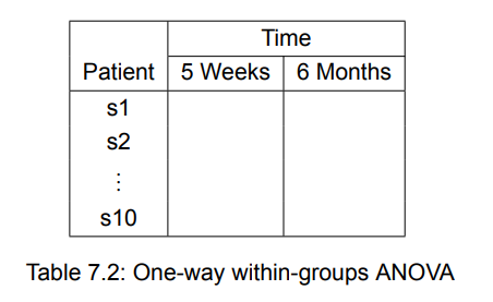
If you are interested in the effect of CBT on anxiety over time, you could place 9 patients in the CBT group and assess them at the end of therapy and again 6 months later.
Time is a within-groups factor with two levels. It’s called a within-groups factor because each patient is measured under both levels.

within-groups ANOVA is also called repeated measures ANOVA.
Hypothesis
\(H_0\) : \(\mu_1 = \mu_2\)
One-way ANOVA
\(Y_{ij}\) is the 𝑗-th observation in the 𝑖-th out of \(𝐾\) groups and \(𝑁\) is the overall sample size, \(n_i\) is the sample size of each group
d.f.1= K - 1
d.f.2 = N - K
The F statistic will be large if the between-group variability is large relative to the within-group variability, which means the mean value of each group is not the same.
F large, reject \(H_0\)
Two-way ANOVA
![[Pasted image 20221128143527.png]]
Therapy (averaged across time), Time (averaged across therapy type) are called the main effects, and the interaction of Therapy and Time called interaction effect.
When you cross two or more factors, as you’ve done here, you have a factorial ANOVA design. Crossing two factors produces a two-way ANOVA, crossing three factors produces a three-way ANOVA, and so forth. When a factorial design includes both between-groups and within-groups factors, it’s also called a mixed-model ANOVA. The current design is a two-way mixed-model factorial ANOVA.
In this case you’ll have three F tests: one for Therapy, one for Time, and one for the Therapy_Time interaction.
The above focus on axiety, however, depression and anxiety often co-occur. Because depression could also explain the group differences on the dependent variable, it’s a confounding factor and its value is a covariate. And if you’re not interested in depression, it’s called a nuisance variable. If you are, then the design would be called an analysis of covariance (ANCOVA)
Finally, you’ve recorded a single dependent variable in this study (the STAI ). You could increase the validity of this study by including additional measures of anxiety (such as family ratings, therapist ratings, and a measure assessing the impact of anxiety on their daily functioning). When there’s more than one dependent variable, the design is called a multivariate analysis of variance (MANOVA). If there are covariates present, it’s called a multivariate analysis of covariance (MANCOVA).
Implementation with R
aov()
- usage:
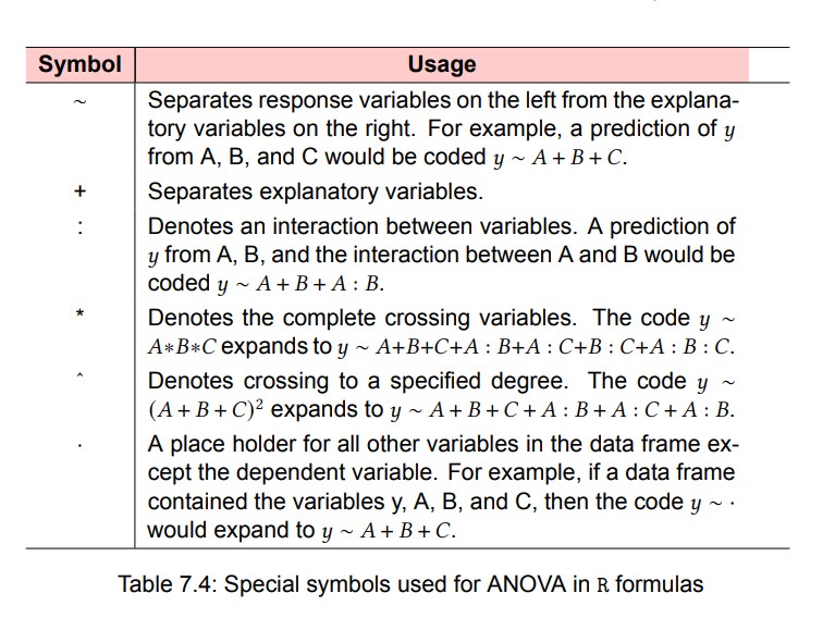
aov(formula, data = dataframe) - symbols-used-for-ANOVA-in-R-formulas

-
Below are formulas for several common research designs. In this table, lowercase letters are quantitative variables, uppercase letters are grouping factors, and Subject is a unique identifier variable for subjects.

-
Type I (sequential) Effects are adjusted for those that appear earlier in the formula. 𝐴 is unadjusted. B is adjusted for the 𝐴. The 𝐴 : 𝐵 interaction is adjusted for 𝐴 and 𝐵.
-
Type II (hierarchical) Effects are adjusted for other effects at the same or lower level. 𝐴 is adjusted for 𝐵. 𝐵 is adjusted for 𝐴. The 𝐴 : 𝐵 interaction is adjusted for both 𝐴 and 𝐵.
-
Type III (marginal) Each effect is adjusted for every other effect in the model. 𝐴 is adjusted for 𝐵 and 𝐴 : 𝐵. 𝐵 is adjusted for 𝐴 and 𝐴 : 𝐵. The 𝐴 : 𝐵 interaction is adjusted for 𝐴 and 𝐵.
R employs the Type I approach by default. Other programs such as SAS and SPSS employ the Type III approach by default.The first model can be written out as 𝑦 ∼ 𝐴 + 𝐵 + 𝐴 : 𝐵. The resulting R ANOVA table will assess
• The impact of 𝐴 on 𝑦
• The impact of 𝐵 on 𝑦, controlling for 𝐴
• The interaction of 𝐴 and 𝐵, controlling for the 𝐴 and 𝐵 main effects.
The greater the imbalance in sample sizes, the greater the impact that the order of the terms will have on the results. In general, more fundamental effects should be listed earlier in the formula. In particular, covariates should be listed first, followed by main effects, followed by two-way interactions, followed by three-way interactions, and so on.
Note that the Anova() function in the car package provides the option of using the Type II or Type III approach, rather than the Type I approach used by the aov() function. You may want to use the Anova() function if you’re concerned about matching your results to those provided by other packages such as SAS and SPSS .
T test
Assumptions
- Independence of observations
- Normality:the distributions of the residuals are normal
- Equality (or "homogeneity") of variances —the variance of data in groups should be the same.
Analysis of Variance ANOVA 方差分析 vs T test
formulas
ANOVA: $$F = \frac{MST}{MSE} = \frac{\text{Mean sum of squares due to treatment}}{\text{Mean sum of squares due to error}}$$
t-test: 2groups (通常是两种疗法把样本分成两类)
ANOVA: 2 or more groups (one factor 2/3/4...levels (groups) / many factors)
when 2 group, n < 50 t-test; otherwise ANOVA


 浙公网安备 33010602011771号